Inspect Data

Looking at your Data

Arvind V.

2025-08-22

“The most certain sign of wisdom is cheerfulness.”

— Michel de Montaigne, Writer and philosopher

Setting up R Packages

library(tidyverse)
library(mosaic) # Our all-in-one package
library(skimr) # Looking at data
library(visdat) # Mapping missing data
library(naniar) # Missing data visualization and munging
library(janitor) # Clean the data
library(tinytable) # Printing Tables for our data

Plot Fonts and Theme

Code

library(systemfonts)
library(showtext)
## Clean the slate
systemfonts::clear_local_fonts()
systemfonts::clear_registry()
##
showtext_opts(dpi = 96) # set DPI for showtext
sysfonts::font_add(
  family = "Alegreya",
  regular = "../../../../../../fonts/Alegreya-Regular.ttf",
  bold = "../../../../../../fonts/Alegreya-Bold.ttf",
  italic = "../../../../../../fonts/Alegreya-Italic.ttf",
  bolditalic = "../../../../../../fonts/Alegreya-BoldItalic.ttf"
)

sysfonts::font_add(
  family = "Roboto Condensed",
  regular = "../../../../../../fonts/RobotoCondensed-Regular.ttf",
  bold = "../../../../../../fonts/RobotoCondensed-Bold.ttf",
  italic = "../../../../../../fonts/RobotoCondensed-Italic.ttf",
  bolditalic = "../../../../../../fonts/RobotoCondensed-BoldItalic.ttf"
)
showtext_auto(enable = TRUE) # enable showtext
##
theme_custom <- function() {
  theme_bw(base_size = 10) +
    #
    # theme(panel.widths = unit(11, "cm"),
    #       panel.heights = unit(6.79, "cm")) + # Golden Ratio

    theme(
      plot.margin = margin_auto(t = 1, r = 2, b = 1, l = 1, unit = "cm"),
      plot.background = element_rect(
        fill = "bisque",
        colour = "black",
        linewidth = 1
      )
    ) +

    theme_sub_axis(
      title = element_text(
        family = "Roboto Condensed",
        size = 10
      ),
      text = element_text(
        family = "Roboto Condensed",
        size = 8
      )
    ) +

    theme_sub_legend(
      text = element_text(
        family = "Roboto Condensed",
        size = 6
      ),
      title = element_text(
        family = "Alegreya",
        size = 8
      )
    ) +

    theme_sub_plot(
      title = element_text(
        family = "Alegreya",
        size = 14, face = "bold"
      ),
      title.position = "plot",
      subtitle = element_text(
        family = "Alegreya",
        size = 10
      ),
      caption = element_text(
        family = "Alegreya",
        size = 6
      ),
      caption.position = "plot"
    )
}

## Use available fonts in ggplot text geoms too!
ggplot2::update_geom_defaults(geom = "text", new = list(
  family = "Roboto Condensed",
  face = "plain",
  size = 3.5,
  color = "#2b2b2b"
))
ggplot2::update_geom_defaults(geom = "label", new = list(
  family = "Roboto Condensed",
  face = "plain",
  size = 3.5,
  color = "#2b2b2b"
))

ggplot2::update_geom_defaults(geom = "marquee", new = list(
  family = "Roboto Condensed",
  face = "plain",
  size = 3.5,
  color = "#2b2b2b"
))
ggplot2::update_geom_defaults(geom = "text_repel", new = list(
  family = "Roboto Condensed",
  face = "plain",
  size = 3.5,
  color = "#2b2b2b"
))
ggplot2::update_geom_defaults(geom = "label_repel", new = list(
  family = "Roboto Condensed",
  face = "plain",
  size = 3.5,
  color = "#2b2b2b"
))

## Set the theme
ggplot2::theme_set(new = theme_custom())

## tinytable options
options("tinytable_tt_digits" = 2)
options("tinytable_format_num_fmt" = "significant_cell")
options(tinytable_html_mathjax = TRUE)


## Set defaults for flextable
flextable::set_flextable_defaults(font.family = "Roboto Condensed")

How do we eat Data?

We spoke of Experiments and Data Gathering in the first module Nature of Data. This helped us to obtain data.

Our first task is to get acquainted with our data, to check the variables, the size of the dataset, how it is formatted, to eat it, as it were.

We need to inspect the data, to understand what it is telling us. The physical significance of each variable needs to sink in before we can do anything with it.

This is especially important in design, since we may be working in domains that are not within our own range of acqaintance or expertise. It is also an important step in the data analysis process.

What do we look for?

How big is the dataset? How many rows and how many columns? Recall: Rows are observations, and columns are variables in the data
What types of columns do we have? Quant? Qual? How many of each?
What are the variable names()? Are they adequate and memorable?
Is there missing data?

All this inspection will lead to:

Data Cleaning, or Munging
A clean dataset, whose variables we understand the meaning of, and which we will explore all the charts at our disposal.

How do these Inspections Work?

Steps in Data Inspection and Cleaning

Inspection:

Use readr::read_csv() or readr::read_delim() to read the data
Inspect Variables Names: base::names() and dplyr::glimpse()
Discover Data Dimension/Size: base::dim()
Structure of the data: utils::str() [ Optional, but very useful. ]
Look for missing data: visdat::vis_dat() and visdat::vis_miss()

And Munging:

Clean the variable names: janitor::clean_names()
Clean up missing data: naniar::replace_with_na_all()
Make factors and rearrange factors to the left of our table using dplyr::mutate(), dplyr::as.factor(), followed by dplyr::relocate()
Make a cool table for our cleaned data with tinytable::tt() (static) or DT::datatable() (interactive)

Case Study: Fast Food

Since we are about to eat our data, we may begin with the dataset fastfood from the TidyTuesday Project for September 4, 2018.

Read the Data

fastfood <- readr::read_csv("https://vincentarelbundock.github.io/Rdatasets/csv/openintro/fastfood.csv")

Rows: 515 Columns: 18
── Column specification ────────────────────────────────────────────────────────
Delimiter: ","
chr  (3): restaurant, item, salad
dbl (15): rownames, calories, cal_fat, total_fat, sat_fat, trans_fat, choles...

ℹ Use `spec()` to retrieve the full column specification for this data.
ℹ Specify the column types or set `show_col_types = FALSE` to quiet this message.

The output from readr::read_csv() tells us that the data frame contains 515 rows and 18 columns. At this point we can’t tell if there are missing values anywhere, or even if there are badly formatted data values anywhere.

Data Inspection

The Size of our Dataset

We already discover from the read_csv() output that the dataset has 515 rows and 18 columns. We can also use dim() to get this information:

dim(fastfood)

[1] 515  18

This tells us that the dataset has 515 rows and 18 columns.

Variables Names

Again, read_csv() tells us that some columns are character, some are double and some are integer. We can use names() and dplyr::glimpse() to get more information about the variables in the dataset.

base::names(fastfood)

 [1] "rownames"    "restaurant"  "item"        "calories"    "cal_fat"    
 [6] "total_fat"   "sat_fat"     "trans_fat"   "cholesterol" "sodium"     
[11] "total_carb"  "fiber"       "sugar"       "protein"     "vit_a"      
[16] "vit_c"       "calcium"     "salad"

Variable Types

dplyr::glimpse(fastfood)

Rows: 515
Columns: 18
$ rownames    <dbl> 1, 2, 3, 4, 5, 6, 7, 8, 9, 10, 11, 12, 13, 14, 15, 16, 17,…
$ restaurant  <chr> "Mcdonalds", "Mcdonalds", "Mcdonalds", "Mcdonalds", "Mcdon…
$ item        <chr> "Artisan Grilled Chicken Sandwich", "Single Bacon Smokehou…
$ calories    <dbl> 380, 840, 1130, 750, 920, 540, 300, 510, 430, 770, 380, 62…
$ cal_fat     <dbl> 60, 410, 600, 280, 410, 250, 100, 210, 190, 400, 170, 300,…
$ total_fat   <dbl> 7, 45, 67, 31, 45, 28, 12, 24, 21, 45, 18, 34, 20, 34, 8, …
$ sat_fat     <dbl> 2.0, 17.0, 27.0, 10.0, 12.0, 10.0, 5.0, 4.0, 11.0, 21.0, 4…
$ trans_fat   <dbl> 0.0, 1.5, 3.0, 0.5, 0.5, 1.0, 0.5, 0.0, 1.0, 2.5, 0.0, 1.5…
$ cholesterol <dbl> 95, 130, 220, 155, 120, 80, 40, 65, 85, 175, 40, 95, 125, …
$ sodium      <dbl> 1110, 1580, 1920, 1940, 1980, 950, 680, 1040, 1040, 1290, …
$ total_carb  <dbl> 44, 62, 63, 62, 81, 46, 33, 49, 35, 42, 38, 48, 48, 67, 31…
$ fiber       <dbl> 3, 2, 3, 2, 4, 3, 2, 3, 2, 3, 2, 3, 3, 5, 2, 2, 3, 3, 5, 2…
$ sugar       <dbl> 11, 18, 18, 18, 18, 9, 7, 6, 7, 10, 5, 11, 11, 11, 6, 3, 1…
$ protein     <dbl> 37, 46, 70, 55, 46, 25, 15, 25, 25, 51, 15, 32, 42, 33, 13…
$ vit_a       <dbl> 4, 6, 10, 6, 6, 10, 10, 0, 20, 20, 2, 10, 10, 10, 2, 4, 6,…
$ vit_c       <dbl> 20, 20, 20, 25, 20, 2, 2, 4, 4, 6, 0, 10, 20, 15, 2, 6, 15…
$ calcium     <dbl> 20, 20, 50, 20, 20, 15, 10, 2, 15, 20, 15, 35, 35, 35, 4, …
$ salad       <chr> "Other", "Other", "Other", "Other", "Other", "Other", "Oth…

By and large, the entries look good. There are no cases, immediately, of character data lurking in Quant variables and such like.

Data Munging

We need to deal with:

Variable Naming
Variable Type conversion
Dealing with Missing Data
Locating Variables for Attention!

Variable Name Options

As a part of the process, we should make sure that the variable names (not entries!!) are formatted in a “clean” way: there are a few options here, such as camelCase, snake_case, kebab-case, or dot.case. We will use the {janitor} package to do this, and also to make sure that the variable names are unique. AND, we will stick with snake_case for the rest of this course.

In this specific case, the variables names look evocative and meaningful enough, without being verbose; they seem just right. But as names in data become complex, with special characters ( %$#@!*_|? etc.), this becomes very useful.

We will also not touch the original data, but save the modified data in a new variable called fast_food_modified. This is a good practice, as it allows us to keep the original data intact, and also to compare the two if needed.

Name Cleaning

fast_food_modified <- fastfood %>%
  janitor::clean_names(case = "snake") # clean names

fast_food_modified

This cleaning up was not needed here, since the original names were already good. But it is a good practice to do this, as it will save you a lot of headaches later on.

Check for Missing Data

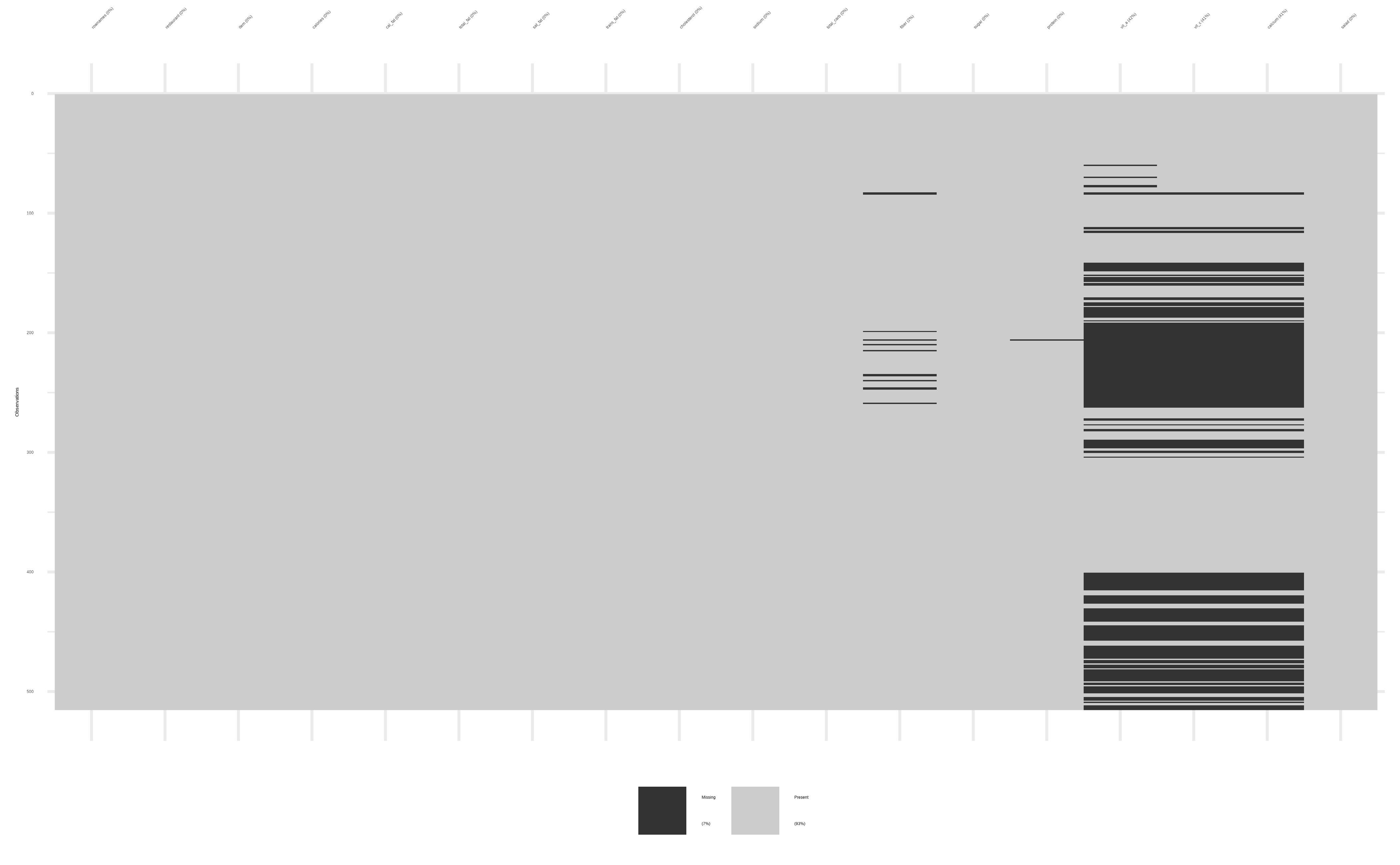
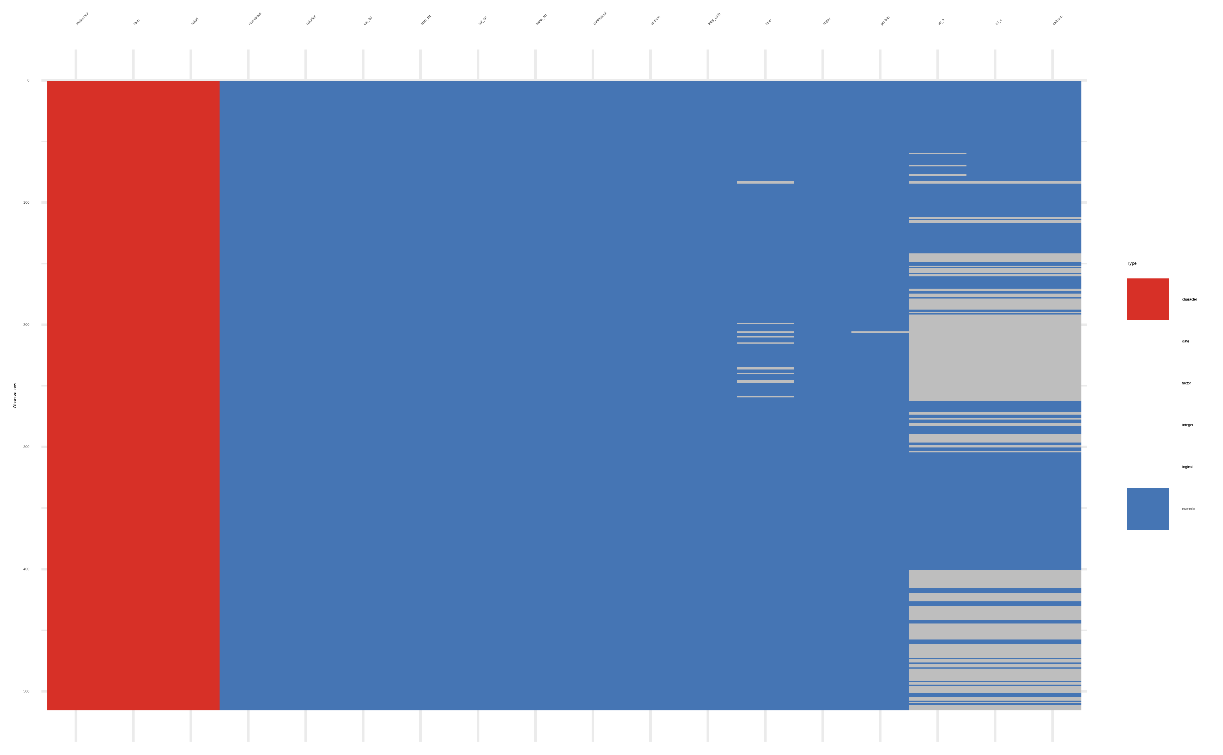
Let us use the {visdat} package to visualize this:

Code

visdat::vis_miss(fastfood)
visdat::vis_dat(fastfood, sort_type = TRUE, palette = "cb_safe")

What to Do with Missing Data

It is clear that there are quite a few missing values in a few columns: vit_a, vit_c and calcium. Some missing values are also present in fiber. So what can one do?

A. Remove rows with missing values: We can use the tidyr::drop_na() command to check for empty locations in a any column, and drop rows containing NA values. Note that this will remove entire rows with missing values in any column, keeping only complete rows. This is a drastic step, and should be done with care.

B. Impute missing values: “Imputation” refers to a technique of inserting data values where they are lacking. This is for a more sophisticated data practitioner, and also requires domain expertise into the subject matter of the dataset itself. We can use the simputation package to impute missing values using various methods, such as trend detection for Quant variables, and using classification for Qual data. This is a more advanced topic, and we will not cover it here.

For our work here, to learn, we will use method A, and simply drop the cells containing NA, whenever we have to.

The `naniar` package

The {naniar} package has two built-in lists for common missing value codes: naniar::common_na_numbers for Quant variables, and naniar::common_na_strings. We can use these to replace these values with NA.

common_na_strings

 [1] "missing" "NA"      "N A"     "N/A"     "#N/A"    "NA "     " NA"    
 [8] "N /A"    "N / A"   " N / A"  "N / A "  "na"      "n a"     "n/a"    
[15] "na "     " na"     "n /a"    "n / a"   " a / a"  "n / a "  "NULL"   
[22] "null"    ""        "\\?"     "\\*"     "\\."

common_na_numbers

[1]    -9   -99  -999 -9999  9999    66    77    88

Replace Missing Values with `NA`

Code

fast_food_modified <- fastfood %>%
  naniar::replace_with_na_all(condition = ~ .x %in% common_na_numbers) %>%
  replace_with_na_all(condition = ~ .x %in% common_na_strings)

glimpse(fast_food_modified)

Rows: 515
Columns: 18
$ rownames    <dbl> 1, 2, 3, 4, 5, 6, 7, 8, 9, 10, 11, 12, 13, 14, 15, 16, 17,…
$ restaurant  <chr> "Mcdonalds", "Mcdonalds", "Mcdonalds", "Mcdonalds", "Mcdon…
$ item        <chr> "Artisan Grilled Chicken Sandwich", "Single Bacon Smokehou…
$ calories    <dbl> 380, 840, 1130, 750, 920, 540, 300, 510, 430, 770, 380, 62…
$ cal_fat     <dbl> 60, 410, 600, 280, 410, 250, 100, 210, 190, 400, 170, 300,…
$ total_fat   <dbl> 7, 45, 67, 31, 45, 28, 12, 24, 21, 45, 18, 34, 20, 34, 8, …
$ sat_fat     <dbl> 2.0, 17.0, 27.0, 10.0, 12.0, 10.0, 5.0, 4.0, 11.0, 21.0, 4…
$ trans_fat   <dbl> 0.0, 1.5, 3.0, 0.5, 0.5, 1.0, 0.5, 0.0, 1.0, 2.5, 0.0, 1.5…
$ cholesterol <dbl> 95, 130, 220, 155, 120, 80, 40, 65, 85, 175, 40, 95, 125, …
$ sodium      <dbl> 1110, 1580, 1920, 1940, 1980, 950, 680, 1040, 1040, 1290, …
$ total_carb  <dbl> 44, 62, 63, 62, 81, 46, 33, 49, 35, 42, 38, 48, 48, 67, 31…
$ fiber       <dbl> 3, 2, 3, 2, 4, 3, 2, 3, 2, 3, 2, 3, 3, 5, 2, 2, 3, 3, 5, 2…
$ sugar       <dbl> 11, 18, 18, 18, 18, 9, 7, 6, 7, 10, 5, 11, 11, 11, 6, 3, 1…
$ protein     <dbl> 37, 46, 70, 55, 46, 25, 15, 25, 25, 51, 15, 32, 42, 33, 13…
$ vit_a       <dbl> 4, 6, 10, 6, 6, 10, 10, 0, 20, 20, 2, 10, 10, 10, 2, 4, 6,…
$ vit_c       <dbl> 20, 20, 20, 25, 20, 2, 2, 4, 4, 6, 0, 10, 20, 15, 2, 6, 15…
$ calcium     <dbl> 20, 20, 50, 20, 20, 15, 10, 2, 15, 20, 15, 35, 35, 35, 4, …
$ salad       <chr> "Other", "Other", "Other", "Other", "Other", "Other", "Oth…

Note that with large datasets, this replacement of strings and numbers with naniar::replace_with_na_all() takes a lot of time to execute.

Data Munging

We see that there are certain variables that must be converted to factors for analytics purposes, since they are unmistakably Qualitative in nature. Let us do that now, for use later:

Code

fast_food_modified <- fast_food_modified %>%
  mutate(
    restaurant = as.factor(restaurant),
    salad = as.factor(salad),
    item = as.factor(item)
  ) %>%
  rename("dish" = item) %>% # rename item to dish

  # arrange the Qual variables first, Quant next
  dplyr::relocate(where(is.factor), .after = rownames)

glimpse(fast_food_modified)

Rows: 515
Columns: 18
$ rownames    <dbl> 1, 2, 3, 4, 5, 6, 7, 8, 9, 10, 11, 12, 13, 14, 15, 16, 17,…
$ restaurant  <fct> Mcdonalds, Mcdonalds, Mcdonalds, Mcdonalds, Mcdonalds, Mcd…
$ dish        <fct> "Artisan Grilled Chicken Sandwich", "Single Bacon Smokehou…
$ salad       <fct> Other, Other, Other, Other, Other, Other, Other, Other, Ot…
$ calories    <dbl> 380, 840, 1130, 750, 920, 540, 300, 510, 430, 770, 380, 62…
$ cal_fat     <dbl> 60, 410, 600, 280, 410, 250, 100, 210, 190, 400, 170, 300,…
$ total_fat   <dbl> 7, 45, 67, 31, 45, 28, 12, 24, 21, 45, 18, 34, 20, 34, 8, …
$ sat_fat     <dbl> 2.0, 17.0, 27.0, 10.0, 12.0, 10.0, 5.0, 4.0, 11.0, 21.0, 4…
$ trans_fat   <dbl> 0.0, 1.5, 3.0, 0.5, 0.5, 1.0, 0.5, 0.0, 1.0, 2.5, 0.0, 1.5…
$ cholesterol <dbl> 95, 130, 220, 155, 120, 80, 40, 65, 85, 175, 40, 95, 125, …
$ sodium      <dbl> 1110, 1580, 1920, 1940, 1980, 950, 680, 1040, 1040, 1290, …
$ total_carb  <dbl> 44, 62, 63, 62, 81, 46, 33, 49, 35, 42, 38, 48, 48, 67, 31…
$ fiber       <dbl> 3, 2, 3, 2, 4, 3, 2, 3, 2, 3, 2, 3, 3, 5, 2, 2, 3, 3, 5, 2…
$ sugar       <dbl> 11, 18, 18, 18, 18, 9, 7, 6, 7, 10, 5, 11, 11, 11, 6, 3, 1…
$ protein     <dbl> 37, 46, 70, 55, 46, 25, 15, 25, 25, 51, 15, 32, 42, 33, 13…
$ vit_a       <dbl> 4, 6, 10, 6, 6, 10, 10, 0, 20, 20, 2, 10, 10, 10, 2, 4, 6,…
$ vit_c       <dbl> 20, 20, 20, 25, 20, 2, 2, 4, 4, 6, 0, 10, 20, 15, 2, 6, 15…
$ calcium     <dbl> 20, 20, 50, 20, 20, 15, 10, 2, 15, 20, 15, 35, 35, 35, 4, …

Data Dictionary

Using all the above methods, we can now create a data dictionary for the fastfood_modified dataset. This is a good practice, as it helps us to understand the data better, and also to communicate with others about the data.

Quantitiative Data

calories(int): Calories in the dish
calories_from_fat(int): Calories from fat
total_fat_g(dbl): Total fat in grams
saturated_fat_g(dbl): Saturated fat in grams
trans_fat (dbl): Trans fat in grams
cholesterol_mg(int): Cholesterol in milligrams
sodium_mg(int): Sodium in milligrams
carbohydrates_g(dbl): Carbohydrates in grams
fiber_g(dbl): Fiber in grams
sugars_g(dbl): Sugars in grams
protein_g(dbl): Protein in grams
vit_a(int): Vitamin A in % Daily Value
vit_c(int): Vitamin C in % Daily Value
calcium(int): Calcium in % Daily Value
iron(int): Iron in % Daily Value

Qualitative Data

restaurant(fct): Name of the restaurant
item(fct): Name of the dish
salad (fct): Is it a salad? (Yes/No)
rownames(int): Row ID

Data Table for Reporting

It is usually a good idea to make crisp business-like tables to show your data. There are many methods to do this.

Static Table Reporting

For Static Tables ( to be published in reports, papers, etc.), one of the simplest and effective ones is to use the tt set of commands from {tinytable}. (The kable set of commands from the {knitr} and {kableExtra} packages also are a good choice):

Code

fast_food_modified %>%
  head(10) %>%
  tinytable::tt(caption = "Fast Food Dataset (Clean)") %>%
  tinytable::theme_html(class = "table table-hover table-striped table-condensed") %>%
  style_tt(fontsize = 0.8) %>%
  stats::setNames(c("Row ID", "Restaurant", "Dish", "Calories", "Calories from fat", "Total Fat (g)", "Saturated Fat (g)", "Trans Fat (g)", "Cholesterol (mg)", "Sodium (mg)", "Carbohydrates (g)", "Fiber (g)", "Sugars (g)", "Protein (g)", "Vitamin A (% DV)", "Vitamin C (% DV)", "Calcium (% DV)", "Iron (% DV)"))

Table 1: Fastfood Clean Static Data Table ( first 10 rows )

Fast Food Dataset (Clean)
Row ID	Restaurant	Dish	Calories	Calories from fat	Total Fat (g)	Saturated Fat (g)	Trans Fat (g)	Cholesterol (mg)	Sodium (mg)	Carbohydrates (g)	Fiber (g)	Sugars (g)	Protein (g)	Vitamin A (% DV)	Vitamin C (% DV)	Calcium (% DV)	Iron (% DV)
1	Mcdonalds	Artisan Grilled Chicken Sandwich	Other	380	60	7	2	0	95	1110	44	3	11	37	4	20	20
2	Mcdonalds	Single Bacon Smokehouse Burger	Other	840	410	45	17	1.5	130	1580	62	2	18	46	6	20	20
3	Mcdonalds	Double Bacon Smokehouse Burger	Other	1130	600	67	27	3	220	1920	63	3	18	70	10	20	50
4	Mcdonalds	Grilled Bacon Smokehouse Chicken Sandwich	Other	750	280	31	10	0.5	155	1940	62	2	18	55	6	25	20
5	Mcdonalds	Crispy Bacon Smokehouse Chicken Sandwich	Other	920	410	45	12	0.5	120	1980	81	4	18	46	6	20	20
6	Mcdonalds	Big Mac	Other	540	250	28	10	1	80	950	46	3	9	25	10	2	15
7	Mcdonalds	Cheeseburger	Other	300	100	12	5	0.5	40	680	33	2	7	15	10	2	10
8	Mcdonalds	Classic Chicken Sandwich	Other	510	210	24	4	0	65	1040	49	3	6	25	0	4	2
9	Mcdonalds	Double Cheeseburger	Other	430	190	21	11	1	85	1040	35	2	7	25	20	4	15
10	Mcdonalds	Double Quarter Pounder® with Cheese	Other	770	400	45	21	2.5	175	1290	42	3	10	51	20	6	20

Interactive Table Reporting

Dynamic Tables can be easily made using the {DT} package, which allows for sorting, searching, and pagination. This is useful for exploring the data interactively. Here is an example:

Code

fast_food_modified %>%
  DT::datatable(
    style = "default",
    caption = htmltools::tags$caption(
      style = "caption-side: top; text-align: left; color: black; font-size: 100%;", "Fast Food Dataset (Clean)"
    ),
    options = list(pageLength = 10, autoWidth = TRUE)
  ) %>%
  DT::formatStyle(
    columns = names(fast_food_modified),
    fontFamily = "Roboto Condensed",
    fontSize = "12px"
  )

Table 2: Fastfood Clean Dynamic Data Table

Your Turn

See if you can do this for this messy dataset which you can download by clicking on the button below the table:

species	island	bill_len	bill_dep	flipper_len	body_mass	sex	year
Adelie		39.1	18.7	181	3750	male	2007
Adelie	Torgersen	39.5	17.4	186	3800	female	2007
Adelie	Torgersen	40.3	18.0	195	3250	female	2007
Adelie	Torgersen	NA	NA	NA	NA	NA	2007
Adelie	Torgersen	999.0	NA	193	3450	female	2007
Adelie	Torgersen	39.3	20.6	190	3650	male	2007

Save it inside your data folder, and call it penguins_messy.csv. Then read the data in your Quarto document using readr::read_csv("data/penguins-messy.csv) and proceed.

Install the package {tastyR}. It contains two datasets, allrecipes and cuisines. Do a similar inspection and if needed, cleaning/munging of these datasets.

Wait, But Why?

Data Inspection is an essential step in getting to know your data.
The structure and format of your data variables, what they mean, and what they might be telling you, is crucial to Exploring, Analysing, and Modelling with the data.
Data Cleaning is an essential step in the data analysis process.
These steps get much of the headache out of the way, and allow you to focus on the real work of Data Exploration, Data Analysis, and Modelling.
And Data Presentation!!

Conclusion

The first step in data analysis is to get to know your data.
Use readr::read_csv() to read the data.
Use names(), glimpse(), dim(), and str() to get to know the variables in your data.
Use visdat::vis_miss() and vis_dat() to visualize missing data.
Use naniar::replace_with_na_all() to replace missing values with NA. If it runs too slowly, then fall back to tidyr::drop_na(). Strange looking strings, which naniar replaces with ease, may have to be separately searched for and replaced, using a combination of dplyr::mutate() and str_detect().
Use janitor::clean_names() to clean the variable names.
Use tinytable::tt() or DT::datatable() to create tables for your data.

Make these part of your Workflow.

References

Nicholas Tierney. (2024-03-05). Getting Started with naniar. https://cran.r-project.org/web/packages/naniar/vignettes/getting-started-w-naniar.html
Vincent Arel-Bundock. tinytable. https://vincentarelbundock.github.io/tinytable/.
Vincent Arel-Bundock. RDatasets. https://vincentarelbundock.github.io/Rdatasets/.

R Package Citations

Package	Version	Citation
DT	0.34.0	Xie et al. (2025)
janitor	2.2.1	Firke (2024)
messy	0.1.0	Rennie (2024)
naniar	1.1.0	Tierney and Cook (2023)
tinytable	0.13.0	Arel-Bundock (2025)
visdat	0.6.0	Tierney (2017)

Arel-Bundock, Vincent. 2025. tinytable: Simple and Configurable Tables in “HTML,” “LaTeX,” “Markdown,” “Word,” “PNG,” “PDF,” and “Typst” Formats. https://doi.org/10.32614/CRAN.package.tinytable.

Firke, Sam. 2024. janitor: Simple Tools for Examining and Cleaning Dirty Data. https://doi.org/10.32614/CRAN.package.janitor.

Rennie, Nicola. 2024. messy: Create Messy Data from Clean Data Frames. https://doi.org/10.32614/CRAN.package.messy.

Tierney, Nicholas. 2017. “visdat: Visualising Whole Data Frames.” JOSS 2 (16): 355. https://doi.org/10.21105/joss.00355.

Tierney, Nicholas, and Dianne Cook. 2023. “Expanding Tidy Data Principles to Facilitate Missing Data Exploration, Visualization and Assessment of Imputations.” Journal of Statistical Software 105 (7): 1–31. https://doi.org/10.18637/jss.v105.i07.

Xie, Yihui, Joe Cheng, Xianying Tan, and Garrick Aden-Buie. 2025. DT: A Wrapper of the JavaScript Library “DataTables”. https://doi.org/10.32614/CRAN.package.DT.

Inspect Data

Setting up R Packages

Plot Fonts and Theme

How do we eat Data?

What do we look for?

How do these Inspections Work?

Steps in Data Inspection and Cleaning

Case Study: Fast Food

Read the Data

Data Inspection

The Size of our Dataset

Variables Names

Variable Types

Data Munging

Variable Name Options

Name Cleaning

Check for Missing Data

What to Do with Missing Data

The naniar package

Replace Missing Values with NA

Data Munging

Data Dictionary

Data Table for Reporting

Static Table Reporting

Interactive Table Reporting

Your Turn

Wait, But Why?

Conclusion

References

R Package Citations

The `naniar` package

Replace Missing Values with `NA`