library(tidyverse) # Sine qua non
library(mosaic) # Out all-in-one package
library(ggformula) # Graphing package
library(skimr) # Looking at Data
library(janitor) # Clean the data
library(naniar) # Handle missing data
library(visdat) # Visualise missing data
library(tinytable) # Printing Static Tables for our data
library(DT) # Interactive Tables for our data
library(crosstable) # Multiple variable summaries
library(marquee) # For Annotations with Fonts
library(ggrepel) # Repel overlapping text labels in ggplot2
How Many of this and that?
2024-06-23
“No matter what happens in life, be good to people. Being good to people is a wonderful legacy to leave behind.”
— Taylor Swift
Plot Fonts and Theme
Code
library(systemfonts)
library(showtext)
## Clean the slate
systemfonts::clear_local_fonts()
systemfonts::clear_registry()
##
showtext_opts(dpi = 96) # set DPI for showtext
sysfonts::font_add(
  family = "Alegreya",
  regular = "../../../../../../fonts/Alegreya-Regular.ttf",
  bold = "../../../../../../fonts/Alegreya-Bold.ttf",
  italic = "../../../../../../fonts/Alegreya-Italic.ttf",
  bolditalic = "../../../../../../fonts/Alegreya-BoldItalic.ttf"
)

sysfonts::font_add(
  family = "Roboto Condensed",
  regular = "../../../../../../fonts/RobotoCondensed-Regular.ttf",
  bold = "../../../../../../fonts/RobotoCondensed-Bold.ttf",
  italic = "../../../../../../fonts/RobotoCondensed-Italic.ttf",
  bolditalic = "../../../../../../fonts/RobotoCondensed-BoldItalic.ttf"
)
showtext_auto(enable = TRUE) # enable showtext
##
theme_custom <- function() {
  theme_bw(base_size = 10) +

    # theme(panel.widths = unit(11, "cm"),
    #       panel.heights = unit(6.79, "cm")) + # Golden Ratio

    theme(
      plot.margin = margin_auto(t = 1, r = 2, b = 1, l = 1, unit = "cm"),
      plot.background = element_rect(
        fill = "bisque",
        colour = "black",
        linewidth = 1
      )
    ) +

    theme_sub_axis(
      title = element_text(
        family = "Roboto Condensed",
        size = 10
      ),
      text = element_text(
        family = "Roboto Condensed",
        size = 8
      )
    ) +

    theme_sub_legend(
      text = element_text(
        family = "Roboto Condensed",
        size = 6
      ),
      title = element_text(
        family = "Alegreya",
        size = 8
      )
    ) +

    theme_sub_plot(
      title = element_text(
        family = "Alegreya",
        size = 14, face = "bold"
      ),
      title.position = "plot",
      subtitle = element_text(
        family = "Alegreya",
        size = 10
      ),
      caption = element_text(
        family = "Alegreya",
        size = 6
      ),
      caption.position = "plot"
    )
}

## Use available fonts in ggplot text geoms too!
ggplot2::update_geom_defaults(geom = "text", new = list(
  family = "Roboto Condensed",
  face = "plain",
  size = 3.5,
  color = "#2b2b2b"
))
ggplot2::update_geom_defaults(geom = "label", new = list(
  family = "Roboto Condensed",
  face = "plain",
  size = 3.5,
  color = "#2b2b2b"
))

ggplot2::update_geom_defaults(geom = "marquee", new = list(
  family = "Roboto Condensed",
  face = "plain",
  size = 3.5,
  color = "#2b2b2b"
))
ggplot2::update_geom_defaults(geom = "text_repel", new = list(
  family = "Roboto Condensed",
  face = "plain",
  size = 3.5,
  color = "#2b2b2b"
))
ggplot2::update_geom_defaults(geom = "label_repel", new = list(
  family = "Roboto Condensed",
  face = "plain",
  size = 3.5,
  color = "#2b2b2b"
))

## Set the theme
ggplot2::theme_set(new = theme_custom())

## tinytable options
options("tinytable_tt_digits" = 2)
options("tinytable_format_num_fmt" = "significant_cell")
options(tinytable_html_mathjax = TRUE)


## Set defaults for flextable
flextable::set_flextable_defaults(font.family = "Roboto Condensed")
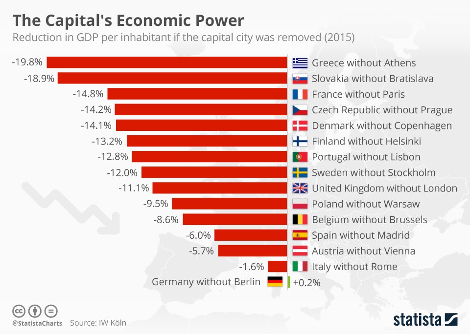
How much does the (financial) capital of a country contribute to its GDP? Which would be India’s city? What would be the reduction in percentage? And these Germans are crazy. (Toc, toc, toc, toc!)
Note how the axis variable that defines the bar locations is a …Qual variable!
ggformula-1

ggplot-1
ggformula-2


ggplot2::theme_set(new = theme_custom())

## Showing "per capita" percentages
taxi_modified %>%
  gf_bar(~local,
    fill = ~tip,
    position = "fill"
  ) %>%
  gf_labs(
    title = "Plot 2C: Filled Bar Chart",
    subtitle = "Shows Per group differences in Proportions!"
  ) %>%
  gf_refine(scale_fill_brewer(palette = "Set1"))
ggplot2::theme_set(new = theme_custom())

## Showing "per capita" percentages
## Better labelling of Y-axis
taxi_modified %>%
  gf_props(~local,
    fill = ~tip,
    position = "fill"
  ) %>%
  gf_labs(
    title = "Plot 2D: Filled Bar Chart",
    subtitle = "Shows Per group differences in Proportions!"
  ) %>%
  gf_refine(scale_fill_brewer(palette = "Set1"))
ggplot-2
Code
ggplot2::theme_set(new = theme_custom())
taxi_modified %>%
ggplot() +
geom_bar(aes(x = local, fill = tip), position = "dodge") +
labs(title = "Plot 2A:Dodged Bar Chart") +
scale_fill_brewer(palette = "Set1")
##
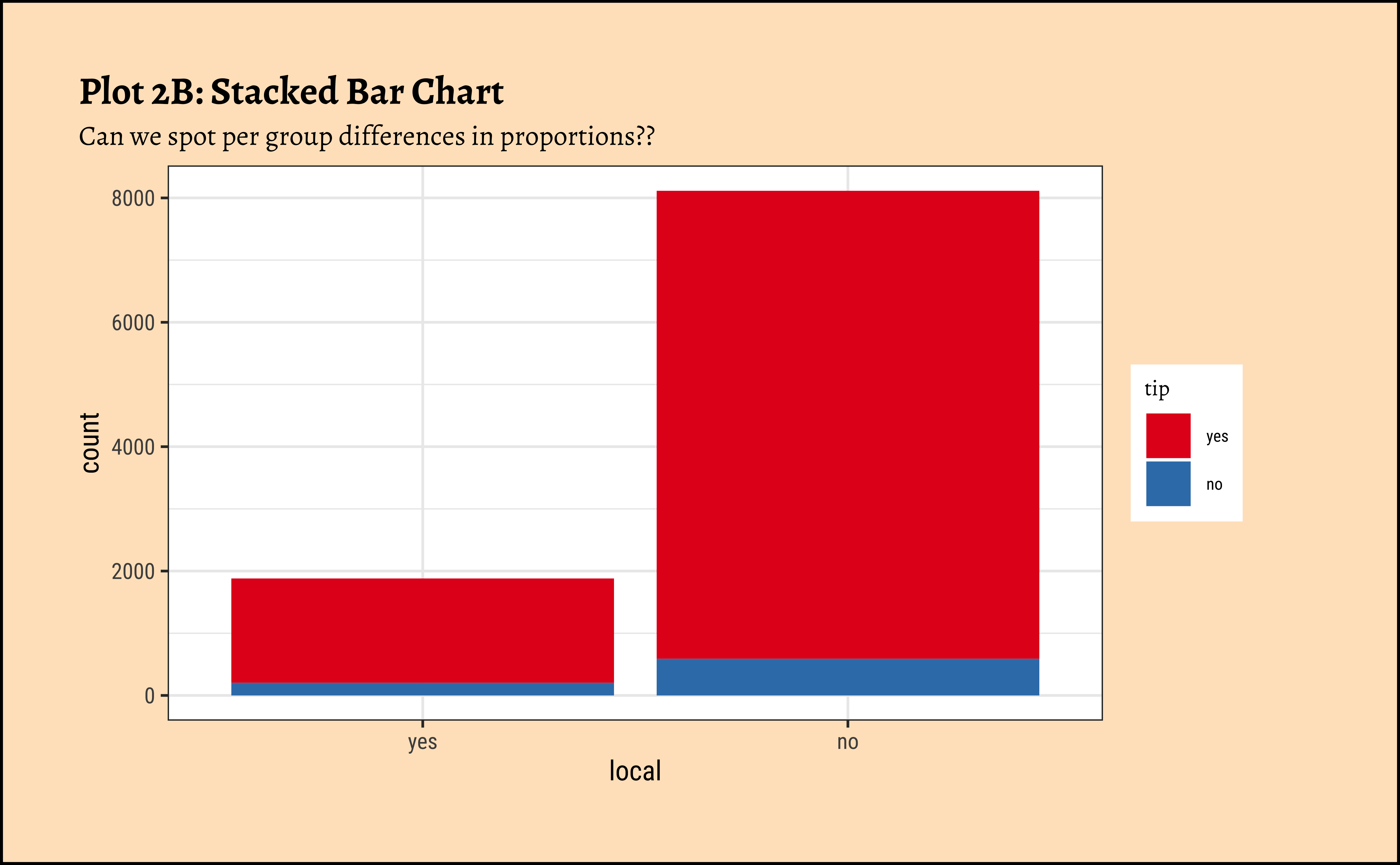
taxi_modified %>%
ggplot() +
geom_bar(aes(x = local, fill = tip), position = "stack") +
labs(
title = "Plot 2B: Stacked Bar Chart",
subtitle = "Can we spot per group differences in proportions??"
) +
scale_fill_brewer(palette = "Set1")
## Showing "per capita" percentages
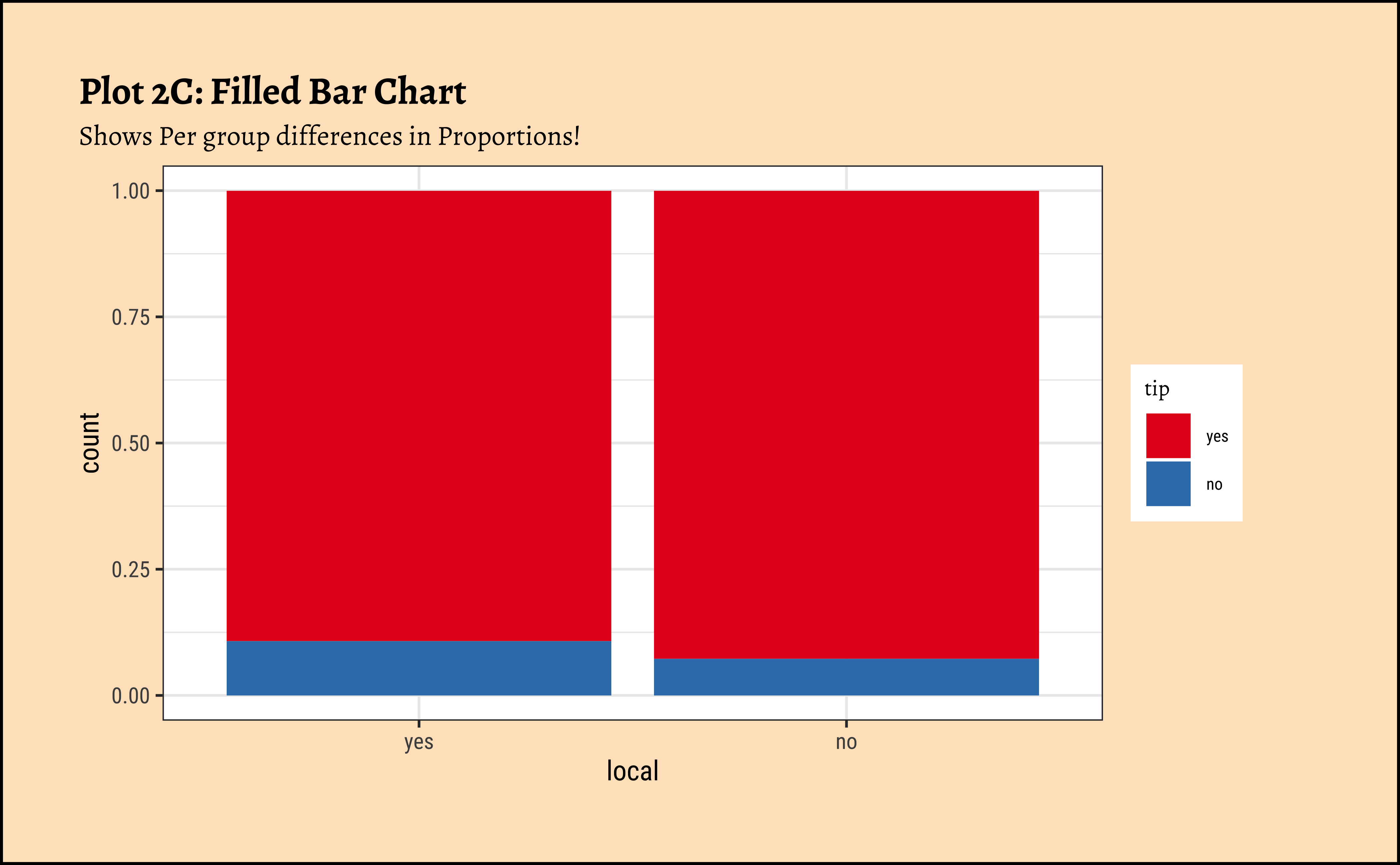
taxi_modified %>%
ggplot() +
geom_bar(aes(x = local, fill = tip), position = "fill") +
labs(title = "Plot 2C: Filled Bar Chart", subtitle = "Shows Per group differences in Proportions!") +
scale_fill_brewer(palette = "Set1")
## Showing "per capita" percentages
## Better labelling of Y-axis
taxi_modified %>%
ggplot() +
geom_bar(aes(x = local, fill = tip), position = "fill") +
labs(
title = "Plot 2D: Filled Bar Chart",
subtitle = "Shows Per group differences in Proportions!",
y = "Proportion"
) +
scale_fill_brewer(palette = "Set1")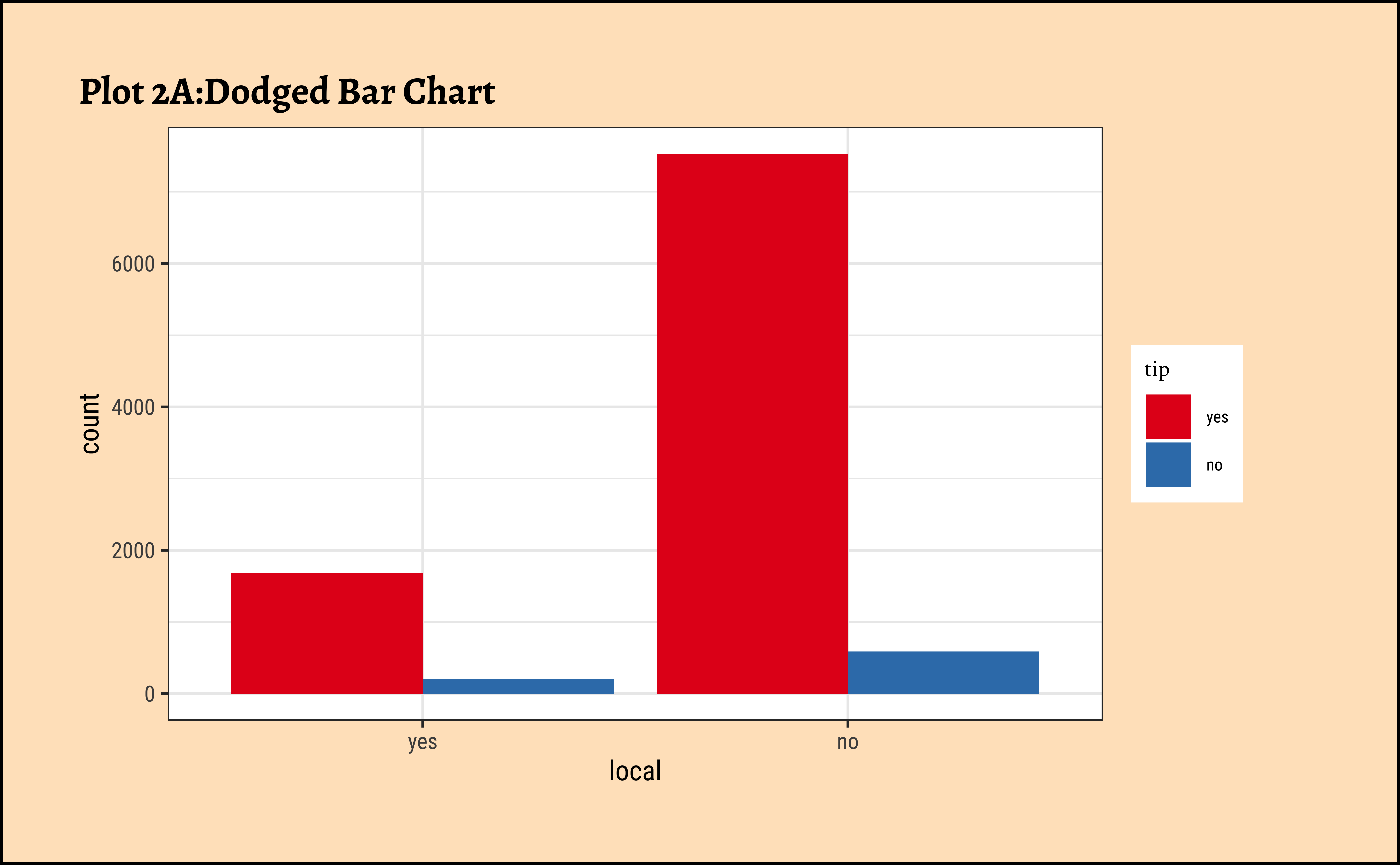

ggformula-3
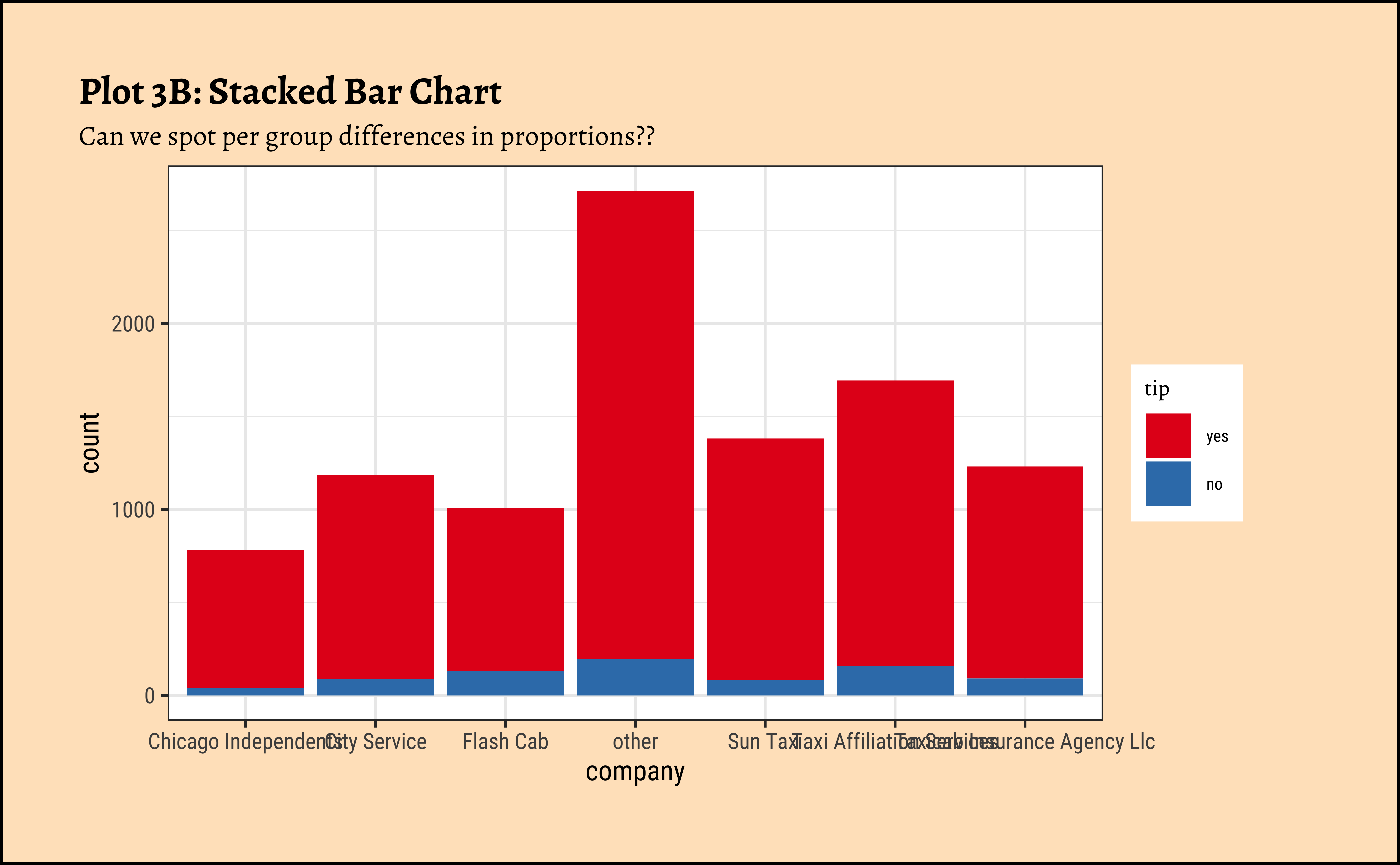
ggplot2::theme_set(new = theme_custom())

taxi_modified %>%
  gf_bar(~company, fill = ~tip, position = "stack") %>%
  gf_labs(
    title = "Plot 3B: Stacked Bar Chart",
    subtitle = "Can we spot per group differences in proportions??"
  ) %>%
  gf_theme(theme(axis.text.x = element_text(size = 6, angle = 45, hjust = 1))) %>%
  gf_refine(scale_fill_brewer(palette = "Set1"))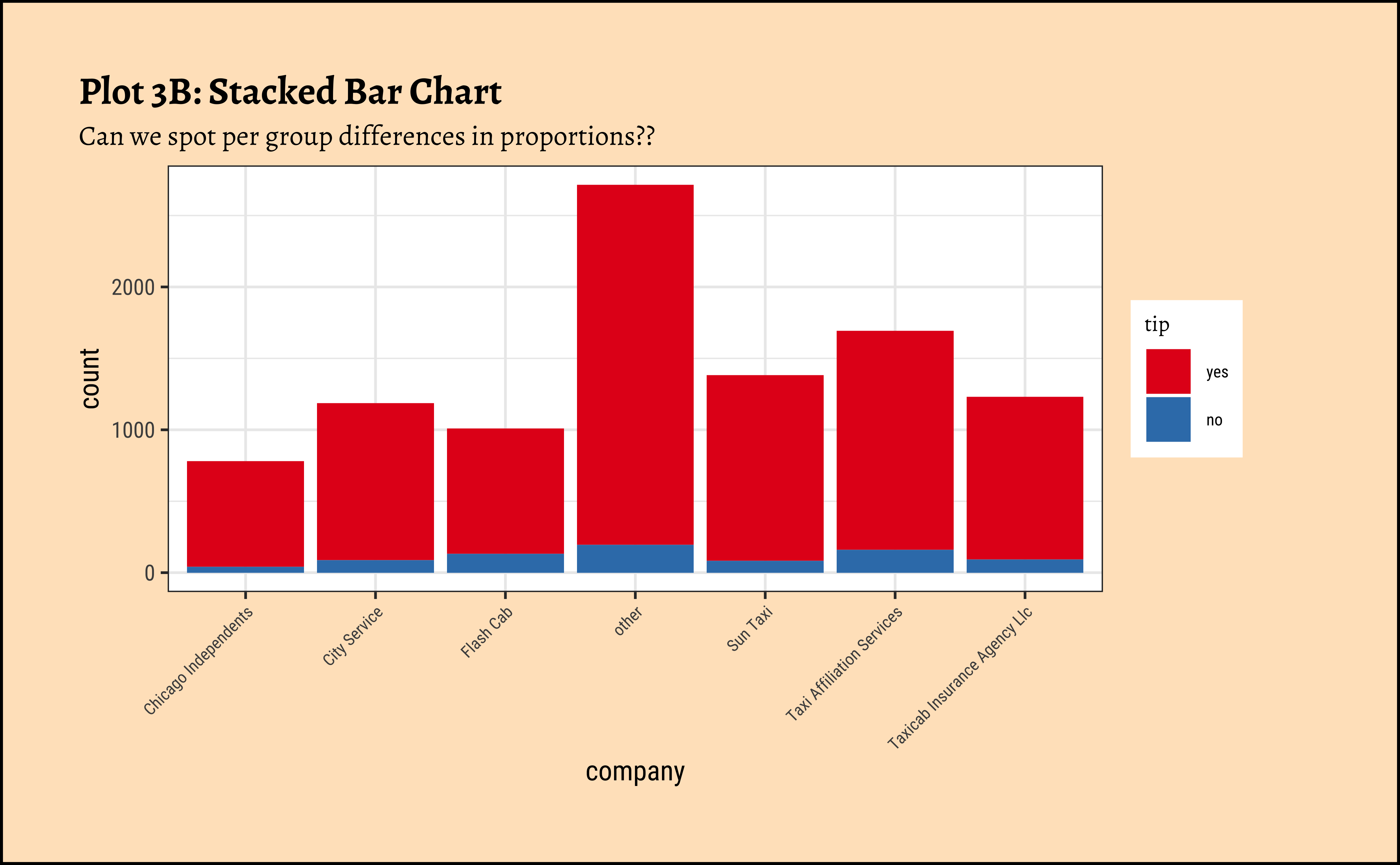
ggplot2::theme_set(new = theme_custom())

## Showing "per capita" percentages
taxi_modified %>%
  gf_percents(~company, fill = ~tip, position = "fill") %>%
  gf_labs(
    title = "Plot 3C: Filled Bar Chart",
    subtitle = "Shows Per group differences in Proportions!"
  ) %>%
  gf_theme(theme(axis.text.x = element_text(size = 6, angle = 45, hjust = 1))) %>%
  gf_refine(scale_fill_brewer(palette = "Set1"))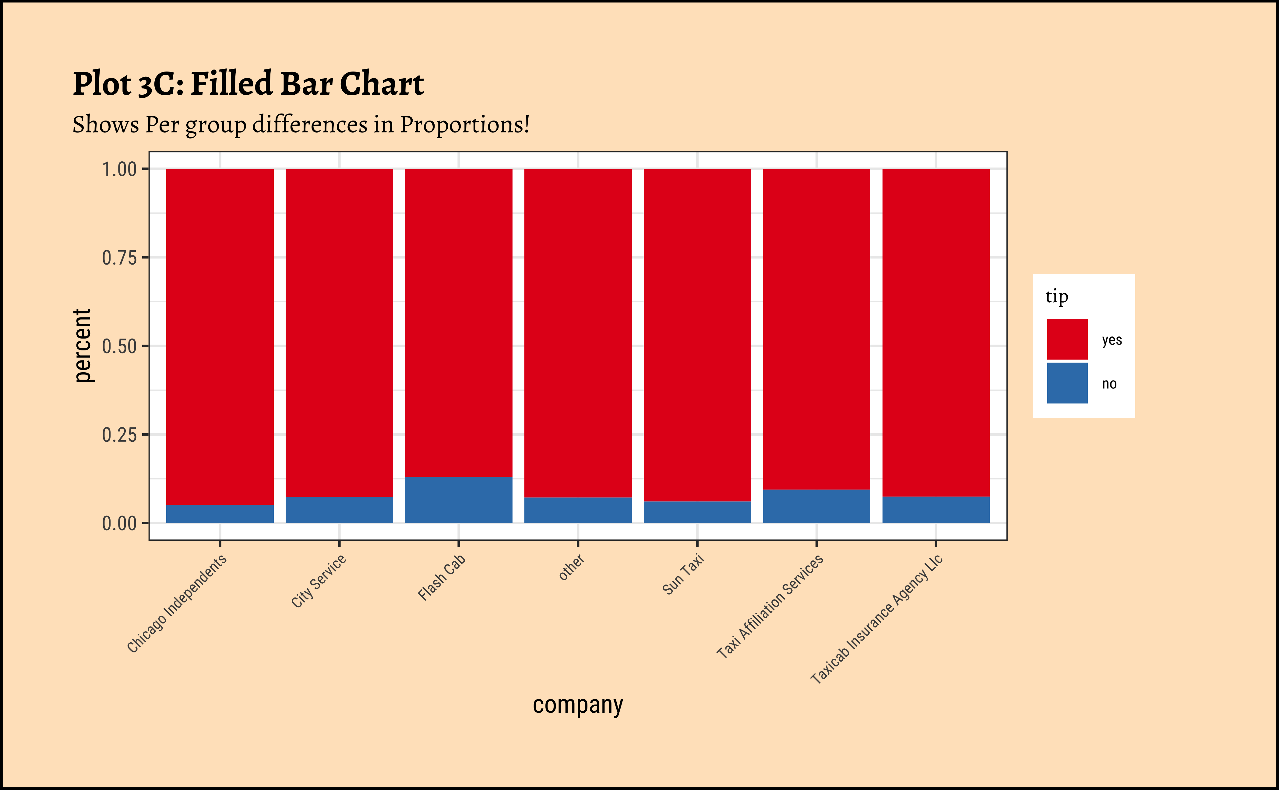
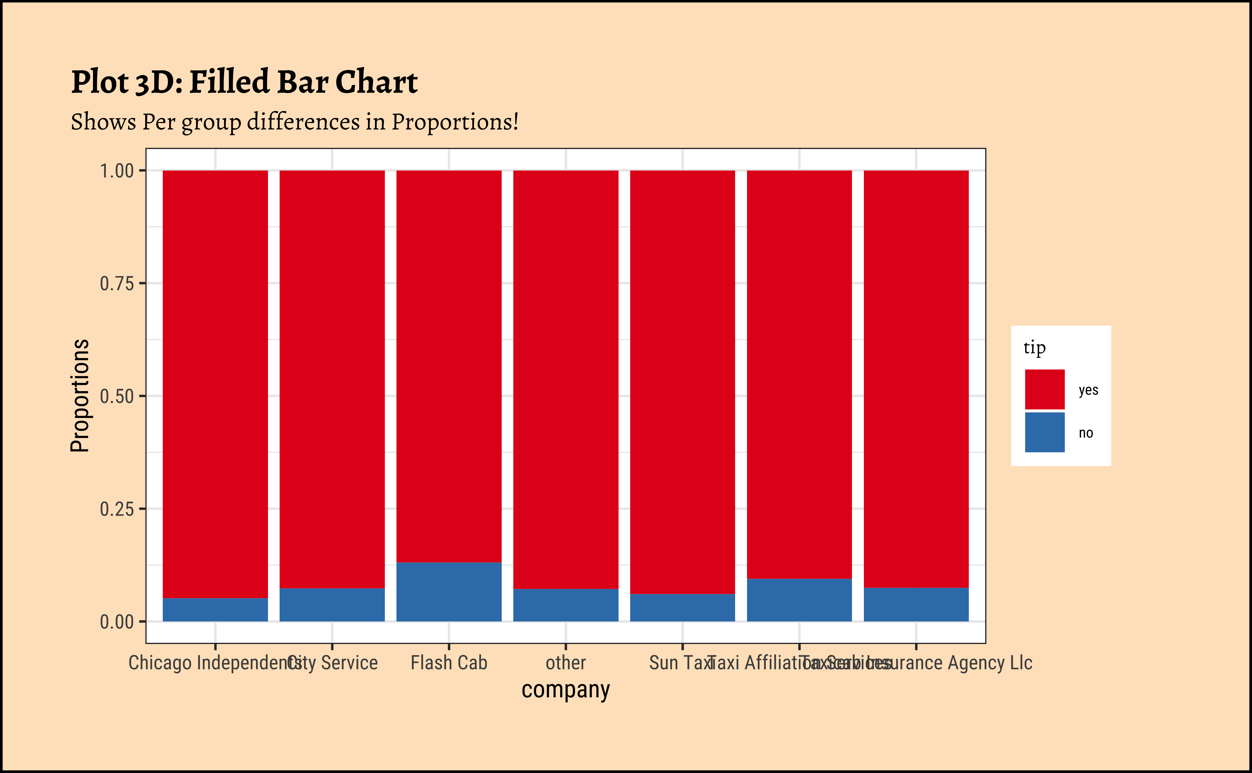
ggplot2::theme_set(new = theme_custom())

## Showing "per capita" percentages
## Better labelling of Y-axis
taxi_modified %>%
  gf_props(~company, fill = ~tip, position = "fill") %>%
  gf_labs(
    title = "Plot 3D: Filled Bar Chart",
    subtitle = "Shows Per group differences in Proportions!"
  ) %>%
  gf_theme(theme(axis.text.x = element_text(size = 6, angle = 45, hjust = 1))) %>%
  gf_refine(scale_fill_brewer(palette = "Set1"))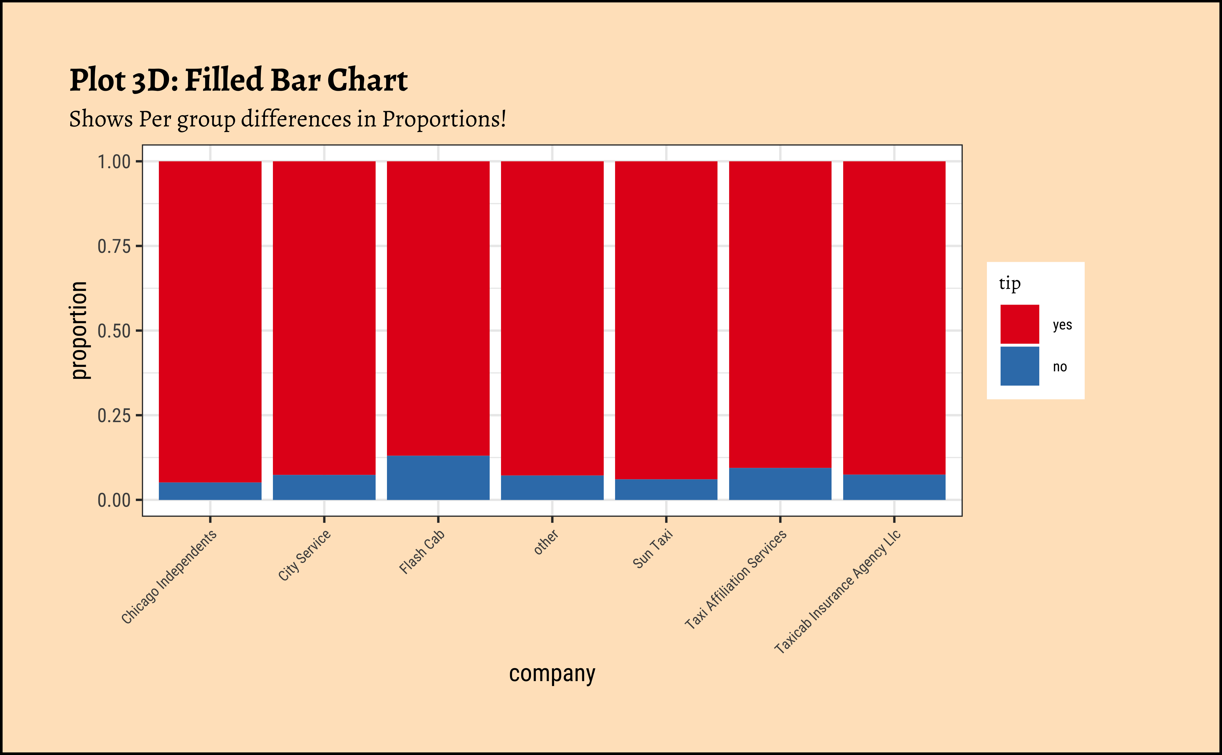
ggplot-3
Code
ggplot2::theme_set(new = theme_custom())
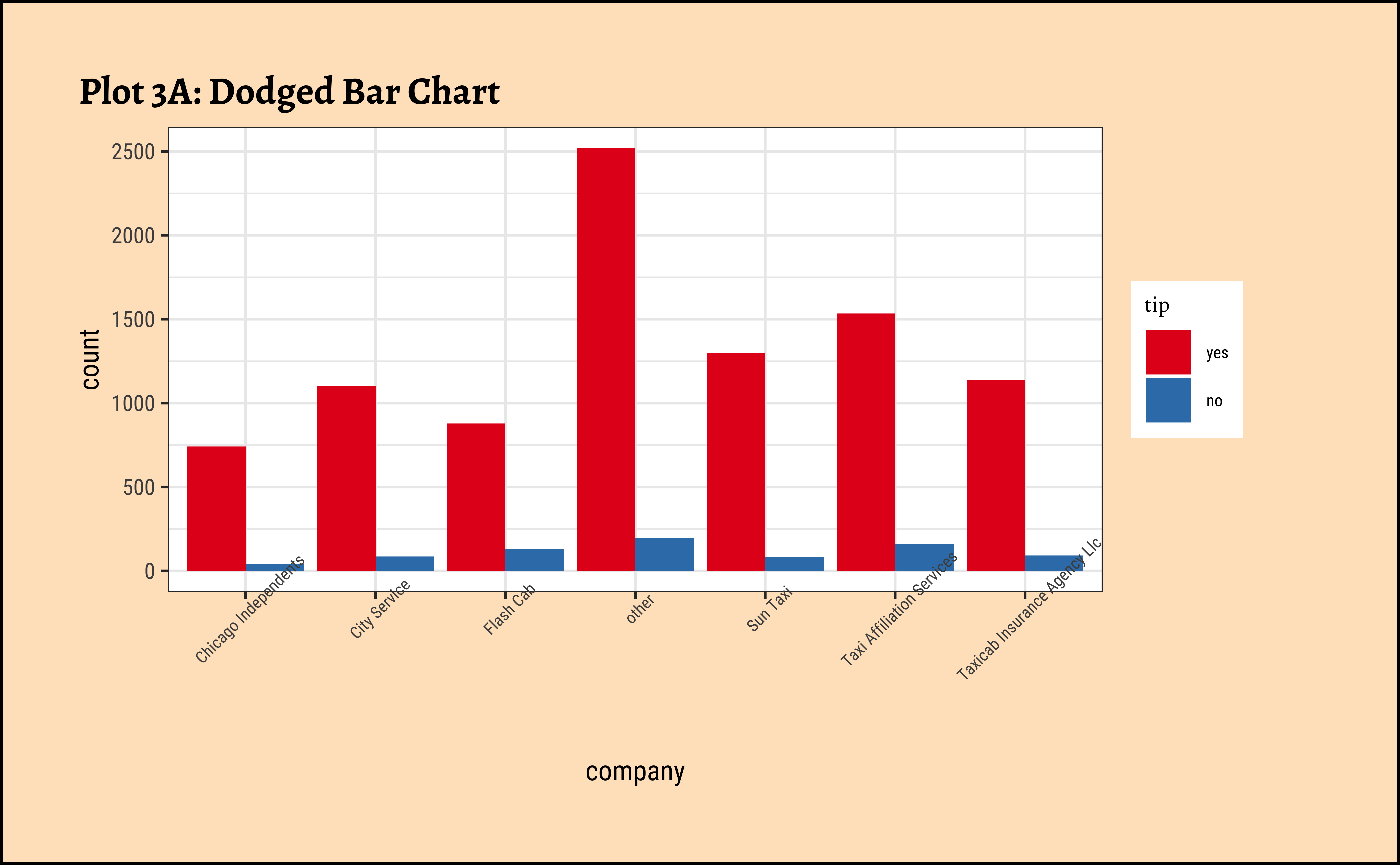
taxi_modified %>%
ggplot() +
geom_bar(aes(x = company, fill = tip), position = "dodge") +
labs(title = "Plot 3A: Dodged Bar Chart") +
theme(theme(axis.text.x = element_text(size = 6, angle = 45, hjust = 1))) +
scale_fill_brewer(palette = "Set1")
##
taxi_modified %>%
ggplot() +
geom_bar(aes(x = company, fill = tip), position = "stack") +
labs(
title = "Plot 3B: Stacked Bar Chart",
subtitle = "Can we spot per group differences in proportions??"
) +
theme(theme(axis.text.x = element_text(size = 6, angle = 45, hjust = 1))) +
scale_fill_brewer(palette = "Set1")
## Showing "per capita" percentages
taxi_modified %>%
ggplot() +
geom_bar(aes(x = company, fill = tip), position = "fill") +
labs(
title = "Plot 3C: Filled Bar Chart",
subtitle = "Shows Per group differences in Proportions!"
) +
theme(theme(axis.text.x = element_text(size = 6, angle = 45, hjust = 1))) +
scale_fill_brewer(palette = "Set1")
## Showing "per capita" percentages
## Better labelling of Y-axis
taxi_modified %>%
ggplot() +
geom_bar(aes(x = company, fill = tip), position = "fill") +
labs(
title = "Plot 3D: Filled Bar Chart",
subtitle = "Shows Per group differences in Proportions!",
y = "Proportions"
) +
theme(theme(axis.text.x = element_text(size = 6, angle = 45, hjust = 1))) +
scale_fill_brewer(palette = "Set1")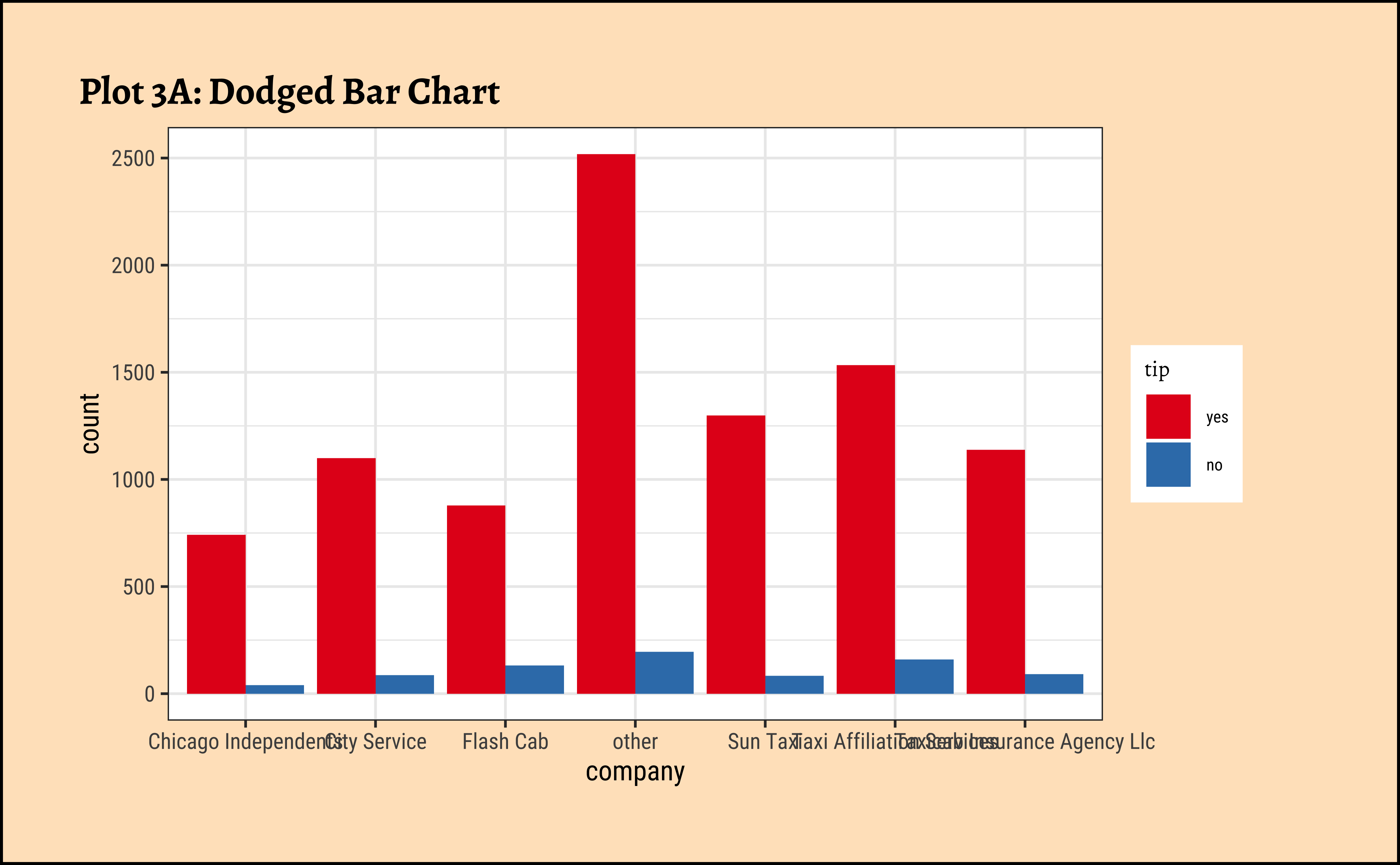

ggformula-4


ggplot2::theme_set(new = theme_custom())
## This may be too busy a graph...
gf_bar(~ dow | hour, fill = ~tip, data = taxi_modified) %>%
gf_labs(
title = "Plot 4E: Counts of Tips by Hour and Day of Week",
subtitle = "Is this plot arrangement easy to grasp?"
) %>%
gf_refine(scale_fill_brewer(palette = "Set1"))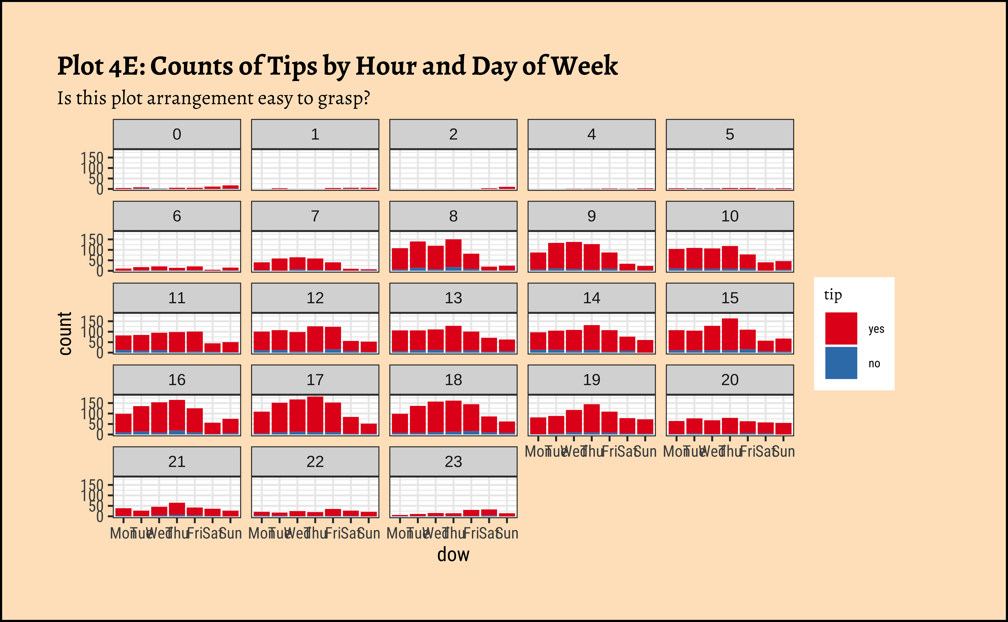
ggplot-4
Code
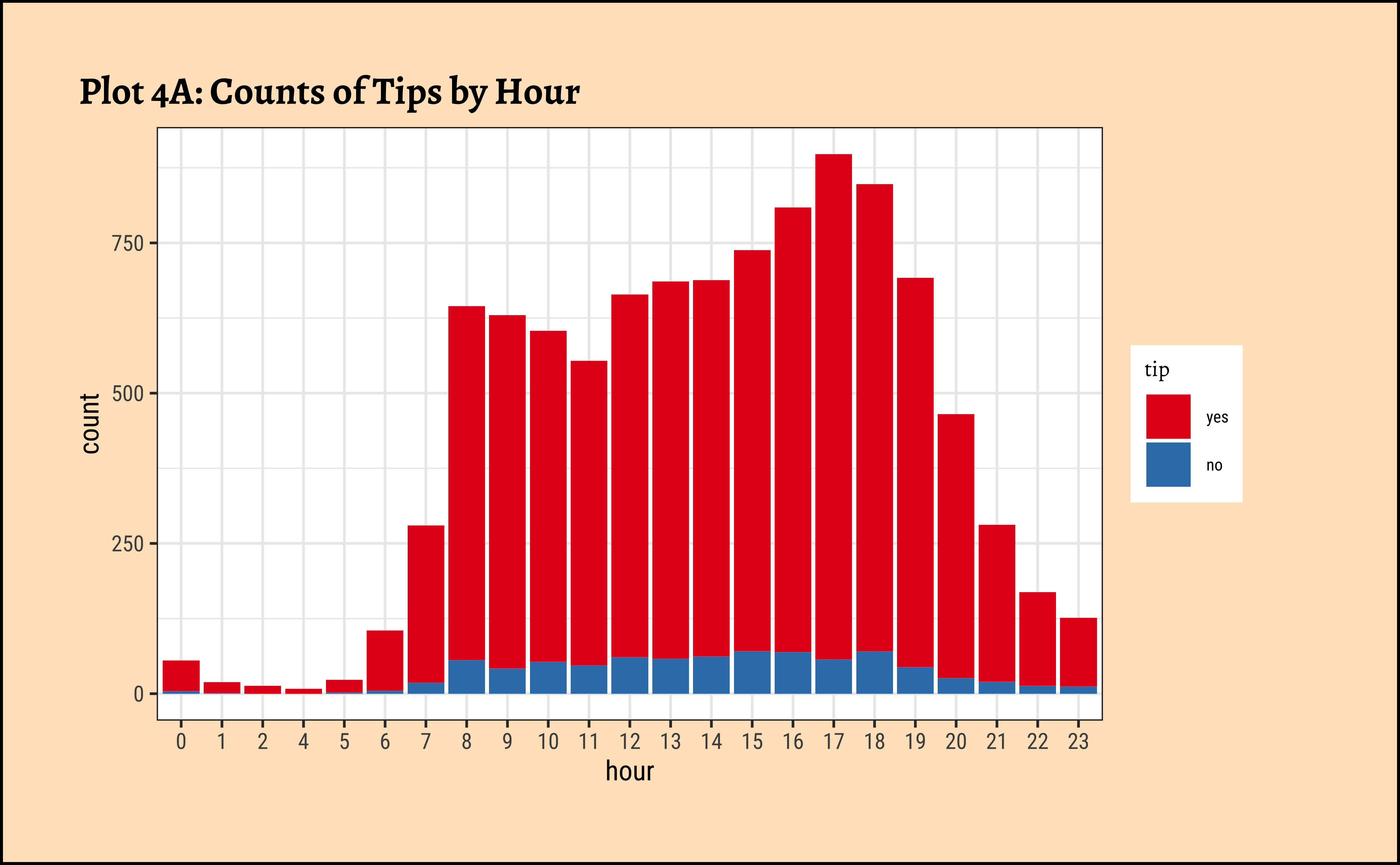
ggplot2::theme_set(new = theme_custom())

gf_bar(~hour, fill = ~tip, data = taxi_modified) %>%
  gf_labs(title = "Plot 4A: Counts of Tips by Hour") %>%
  gf_refine(scale_fill_brewer(palette = "Set1"))
##
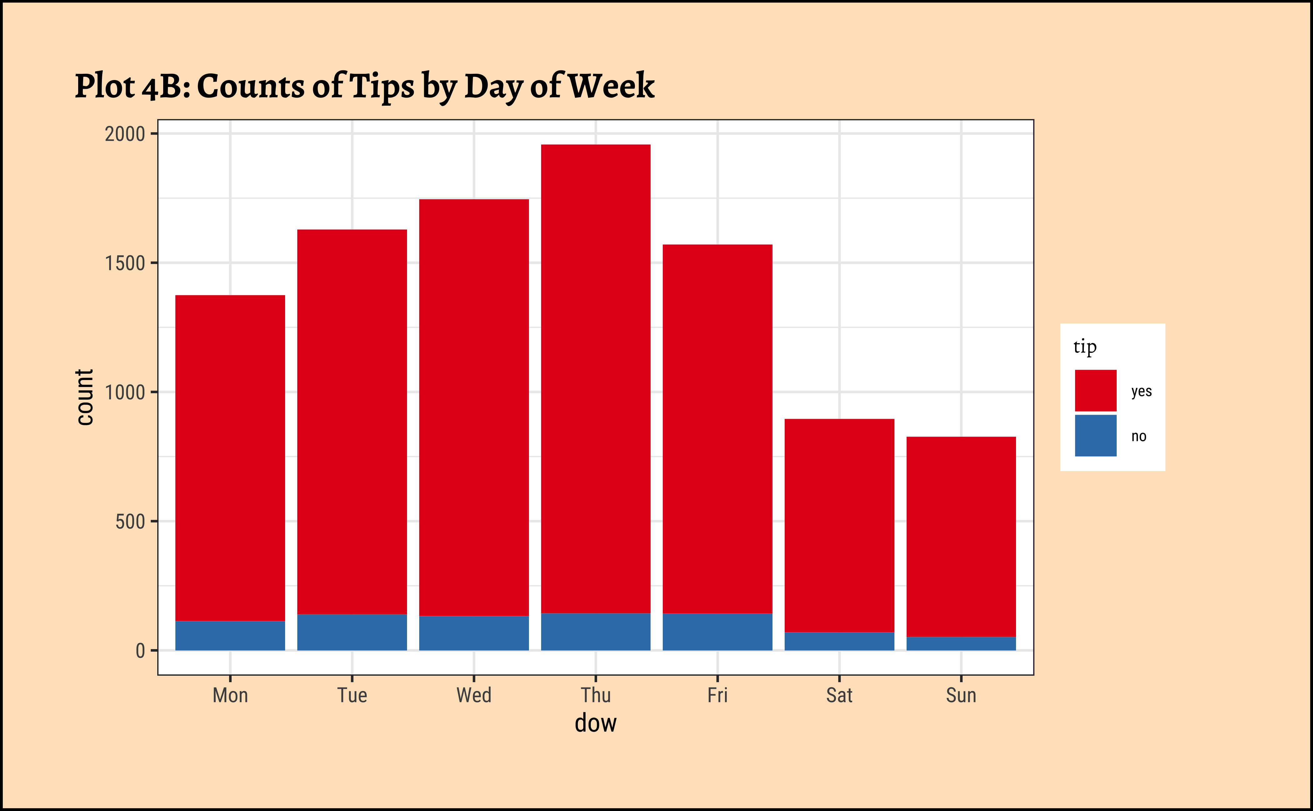
ggplot(taxi_modified) +
geom_bar(aes(x = dow, fill = tip)) +
labs(title = "Plot 4B: Counts of Tips by Day of Week") +
scale_fill_brewer(palette = "Set1")
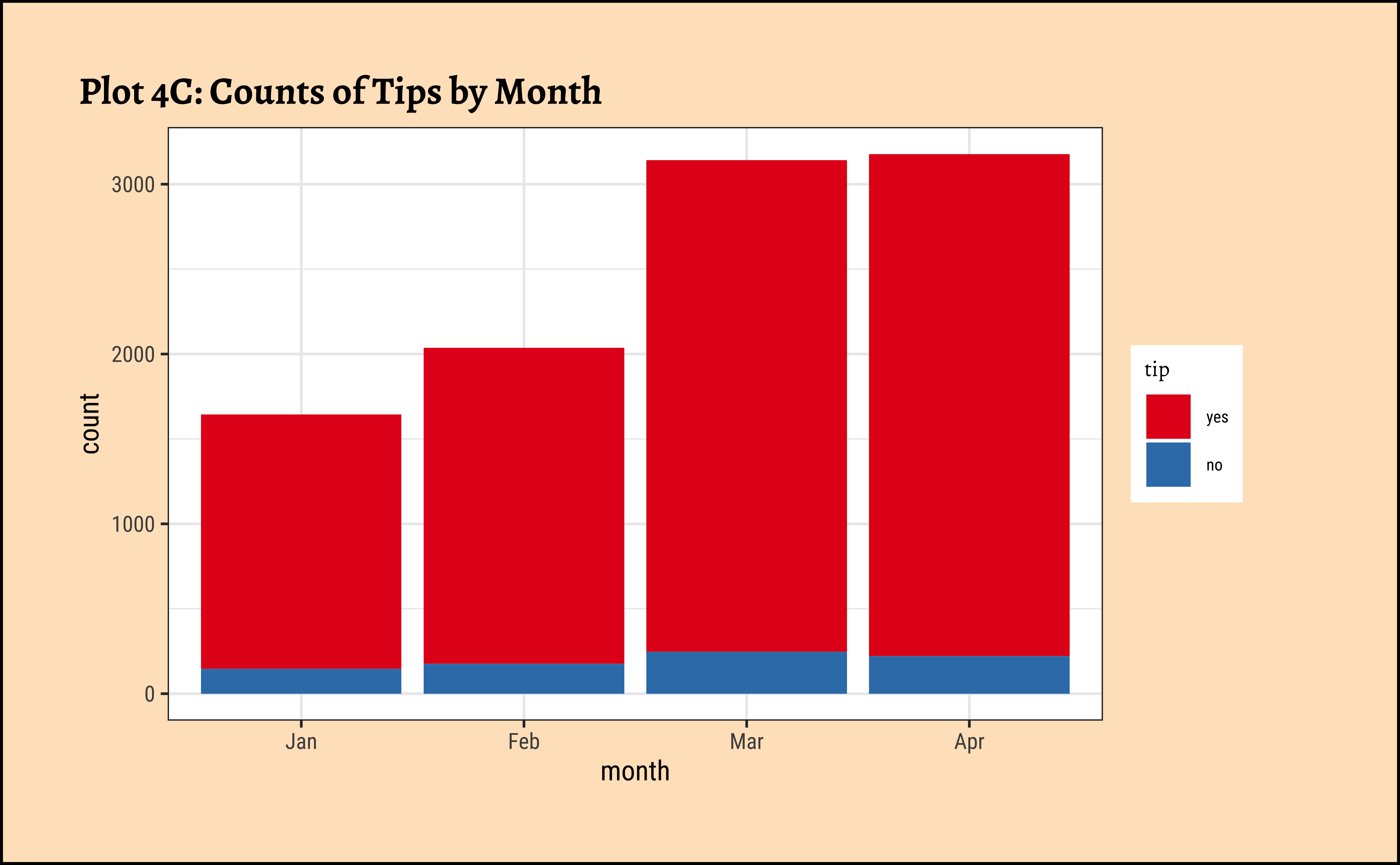
##
ggplot(taxi_modified) +
geom_bar(aes(x = month, fill = tip)) +
labs(title = "Plot 4C: Counts of Tips by Month") +
scale_fill_brewer(palette = "Set1")
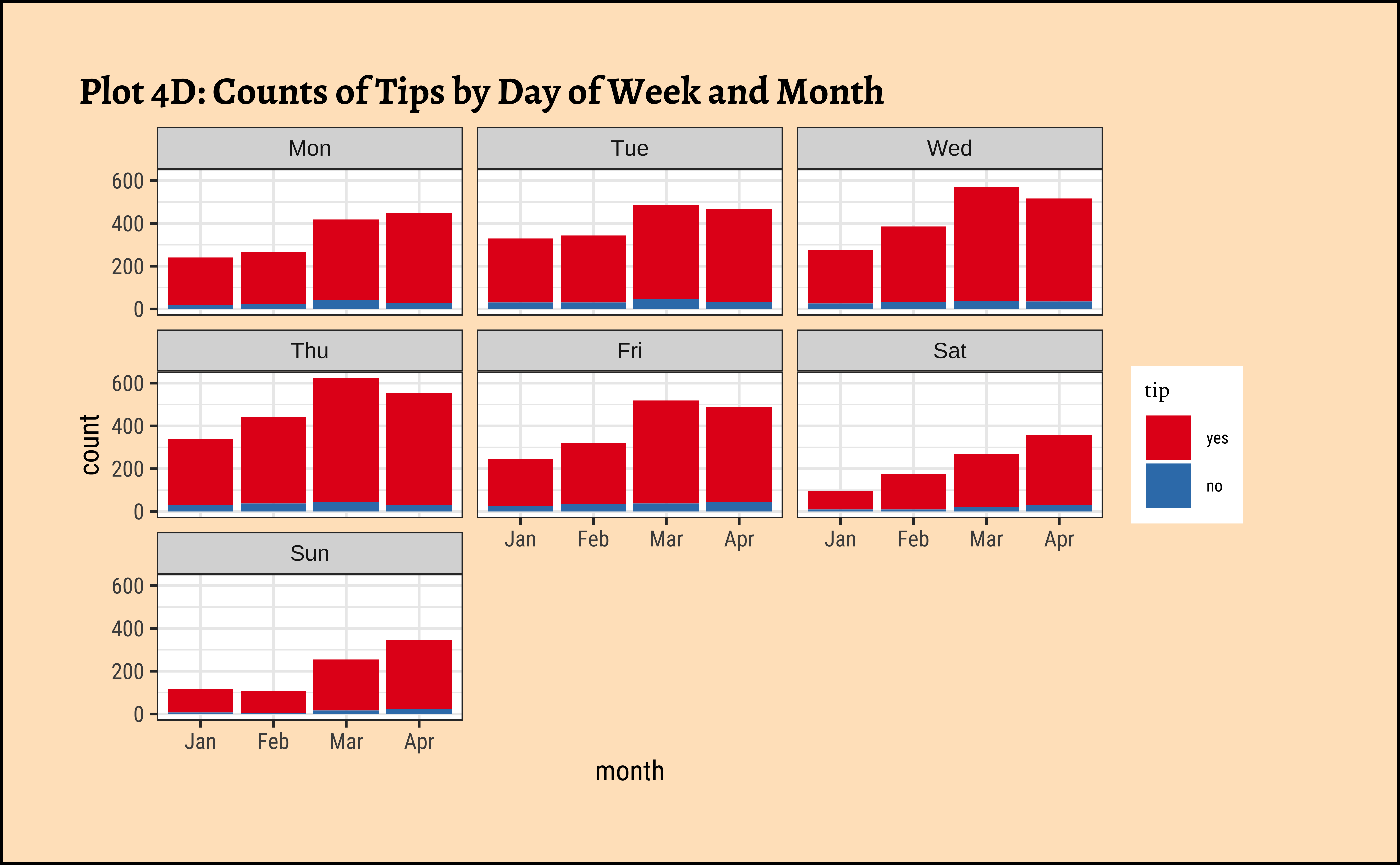
##
ggplot(taxi_modified) +
geom_bar(aes(x = month, fill = tip)) +
facet_wrap(~dow) +
labs(title = "Plot 4D: Counts of Tips by Day of Week and Month") +
scale_fill_brewer(palette = "Set1")
##
ggplot(taxi_modified) +
geom_bar(aes(x = dow, fill = tip)) +
facet_wrap(~hour) +
labs(
title = "Plot 4E: Counts of Tips by Hour and Day of Week",
subtitle = "Is this plot arrangement easy to grasp?"
) +
scale_fill_brewer(palette = "Set1")
##
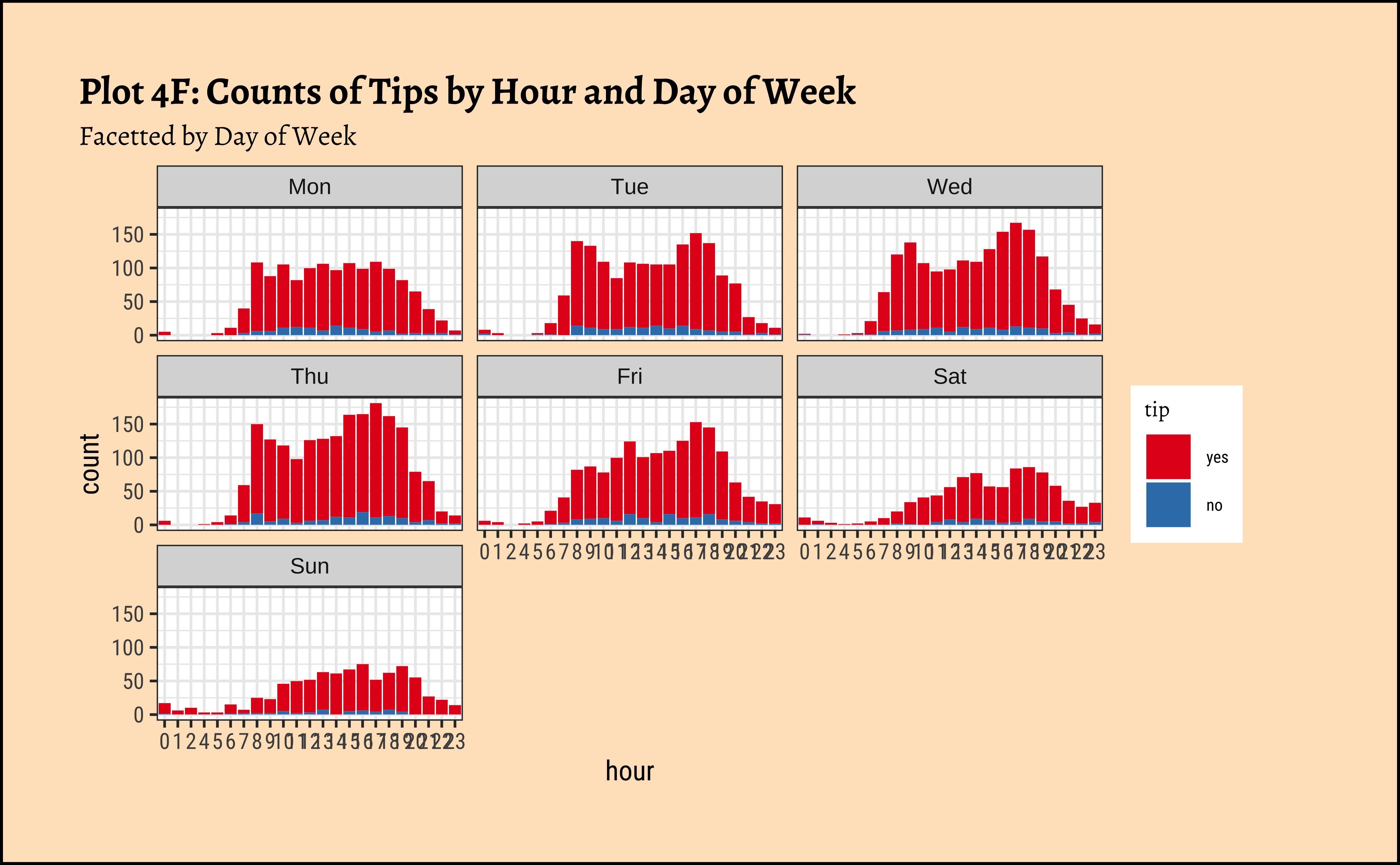
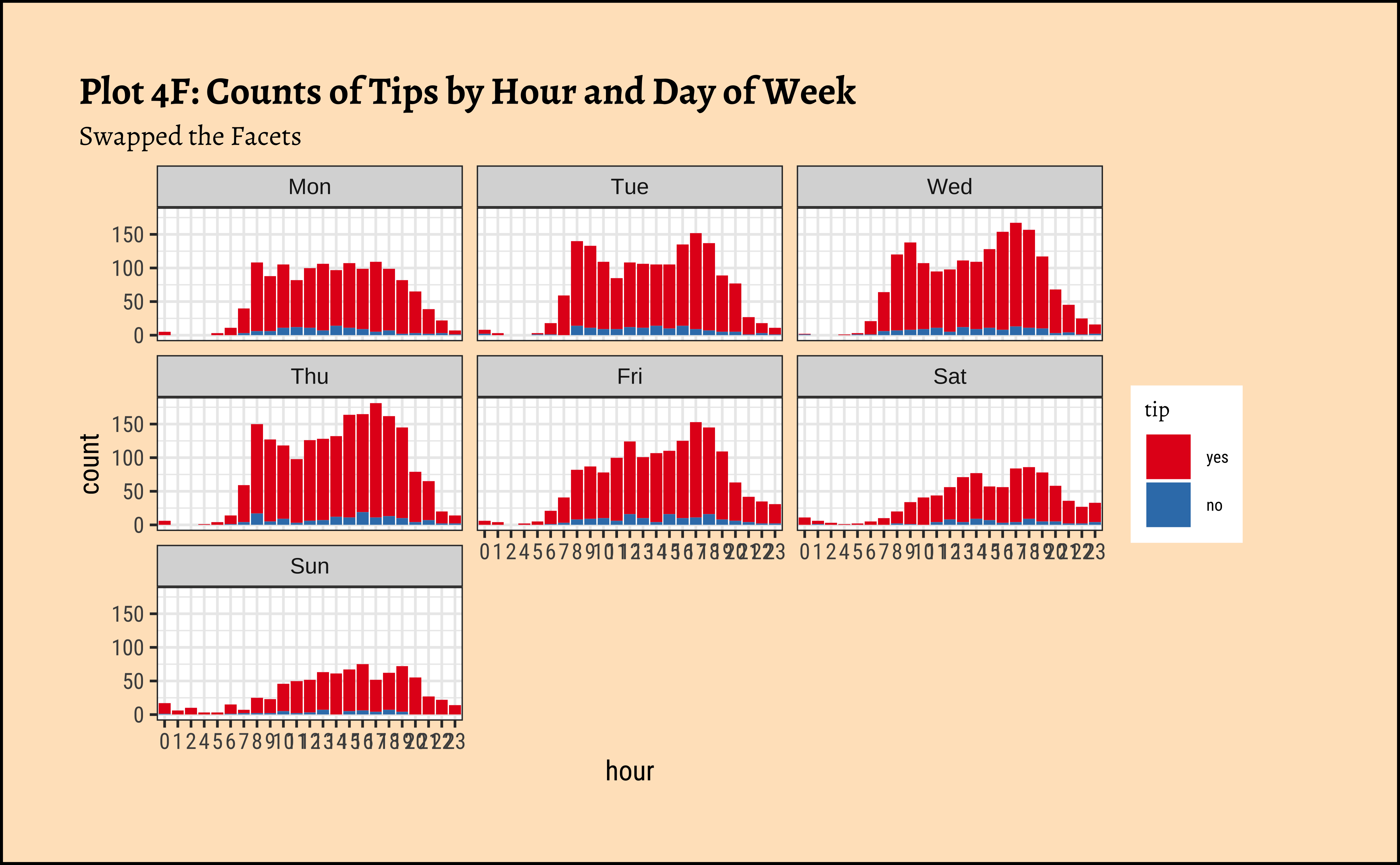
ggplot(taxi_modified) +
geom_bar(aes(x = hour, fill = tip)) +
facet_wrap(~dow) +
labs(
title = "Plot 4F: Counts of Tips by Hour and Day of Week",
subtitle = "Swapped the Facets"
) +
scale_fill_brewer(palette = "Set1")


Proportions and Percentages
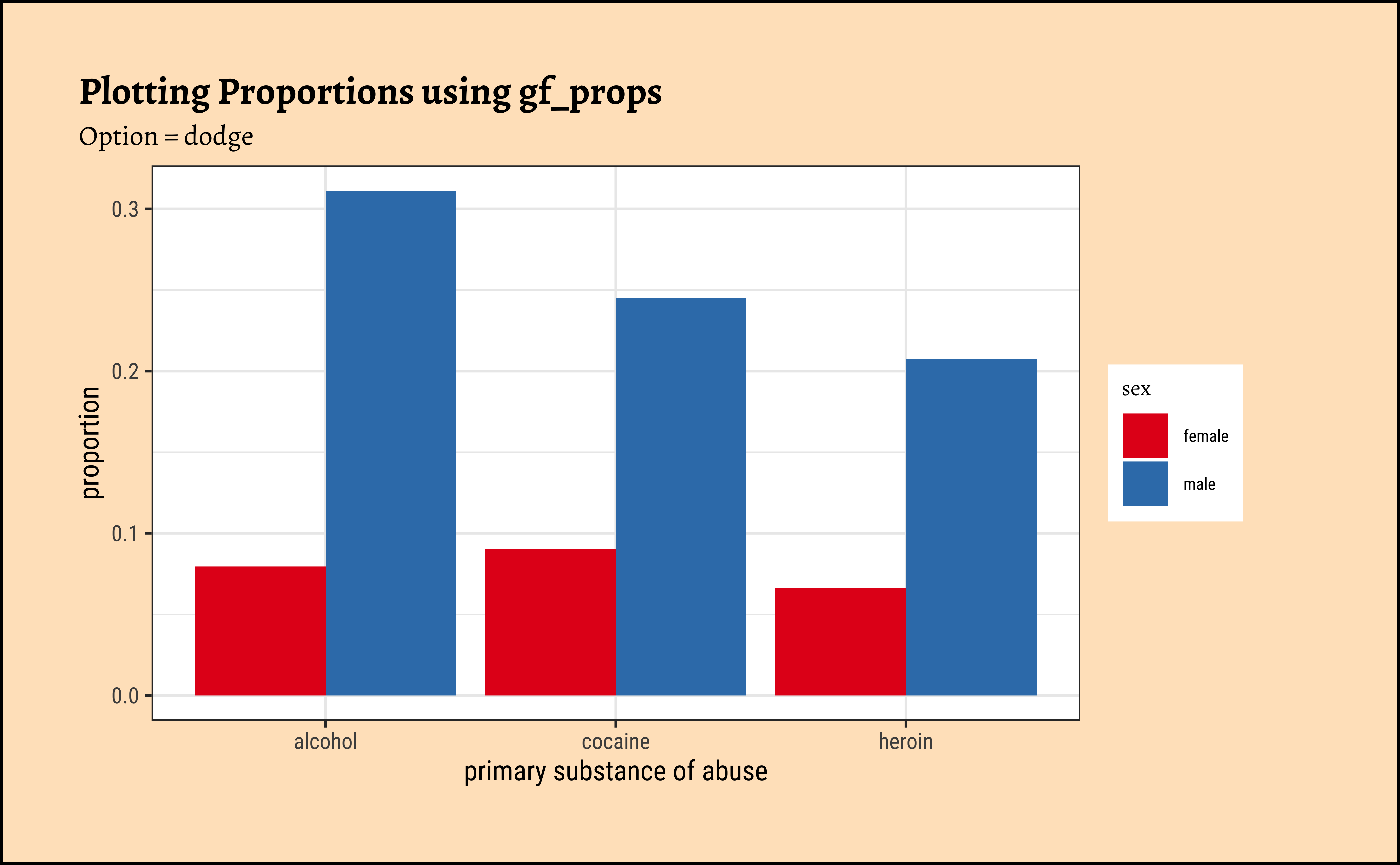
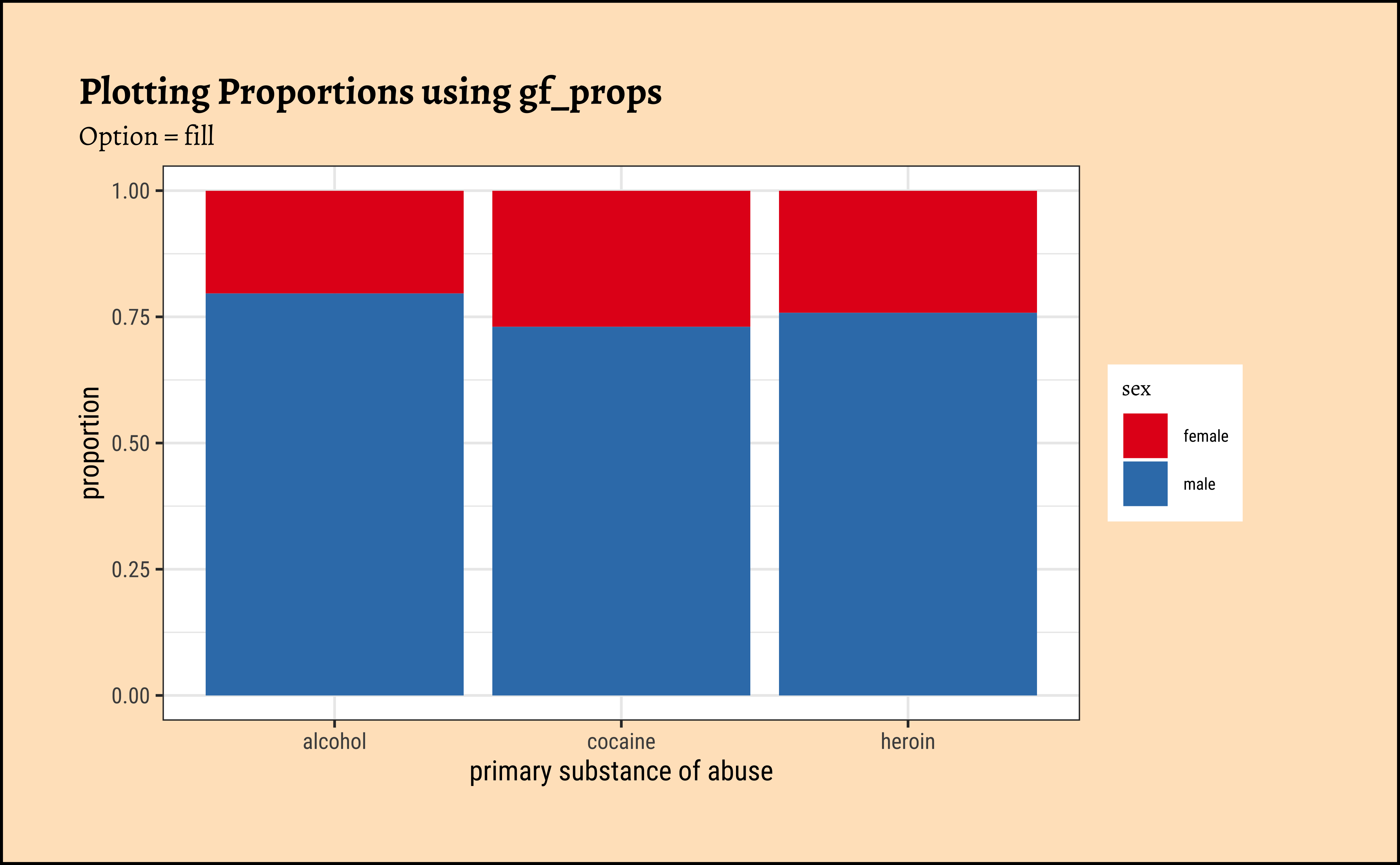
ggplot2::theme_set(new = theme_custom())

gf_percents(~substance,
  data = mosaicData::HELPrct, fill = ~sex,
  position = "dodge"
) %>%
  gf_refine(
    scale_y_continuous(
      labels = scales::label_percent(scale = 1)
    )
  ) %>%
  gf_labs(title = "Plotting Percentages using gf_percents") %>%
  gf_refine(scale_fill_brewer(palette = "Set1"))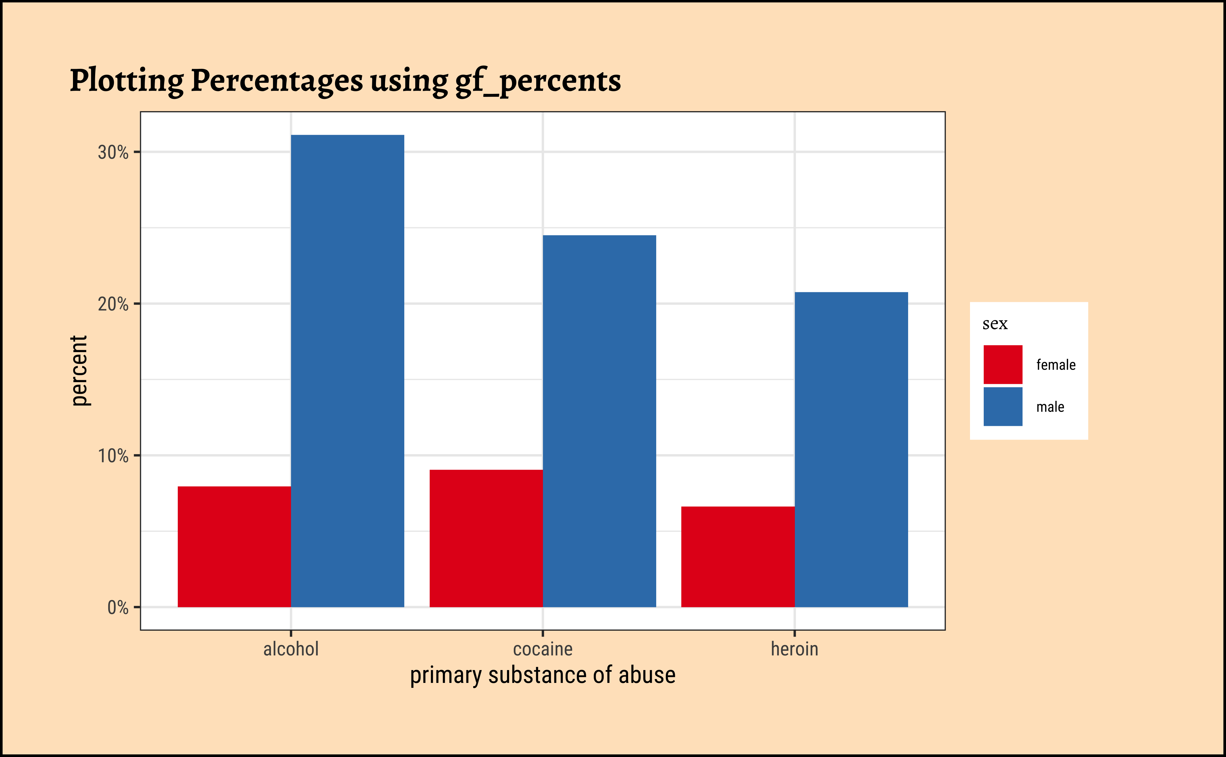
Counts from Literature
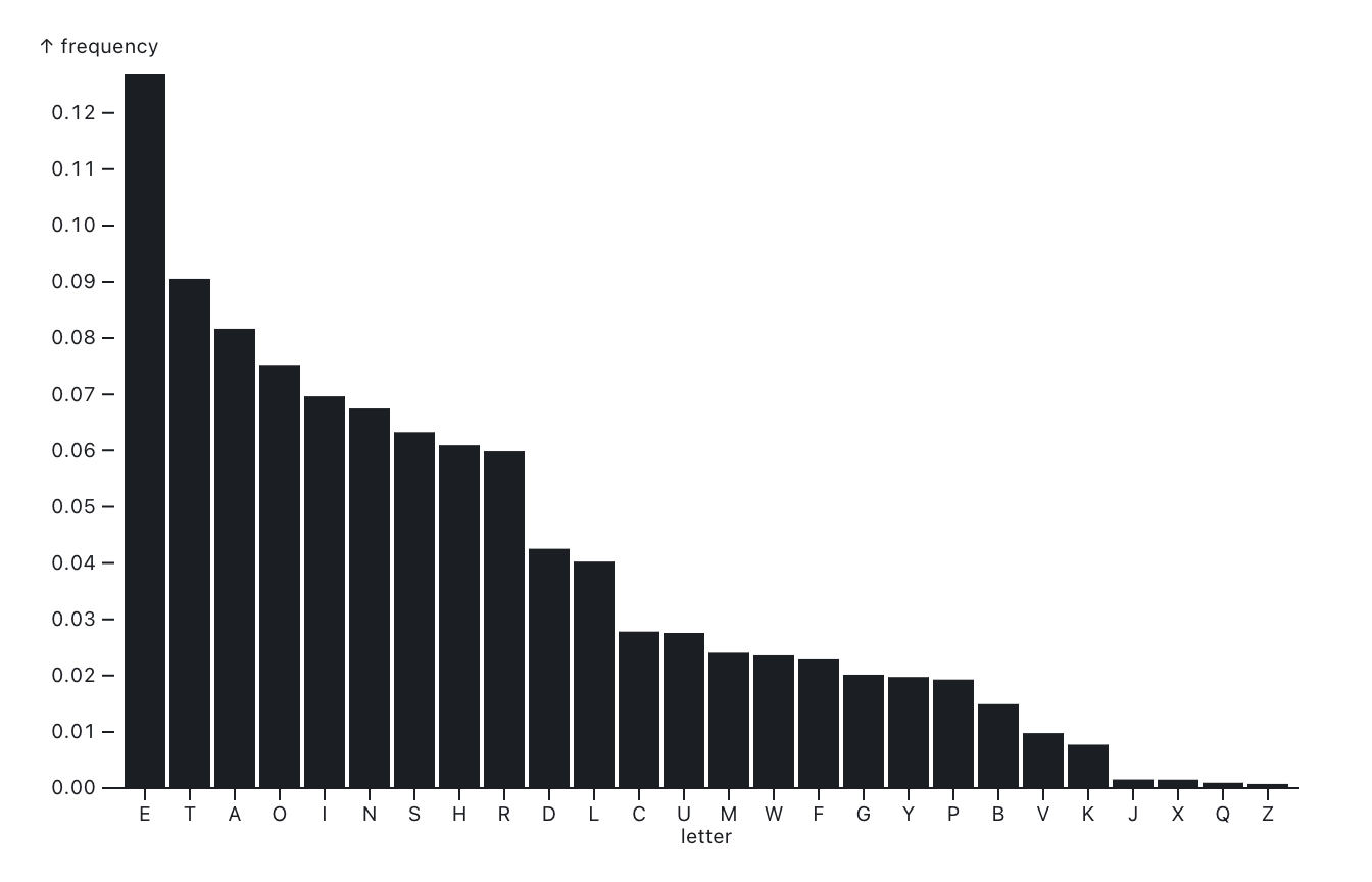
Zipf’s Law
- Since the X-axis in bar charts is Qualitative (the bars don’t touch, remember!) it is possible to sort the bars at will, based on the levels within the Qualitative variables. See the approx Zipf’s Law distribution for the English alphabet above
- In Figure 2, the letters of the alphabet are “levels” within a Qualitative variable
- these levels have been sorted based on the frequency or count!
- This is what Sherlock Holmes might have done,
- Or the method how they cracked the code to the treasure in this story.