🃏 Permutation Test for Two Proportions
Test Proportions
1 Setting up the Packages
2 Introduction
We saw from the diagram created by Allen Downey that there is only one test! We will now use this philosophy to develop a technique that allows us to mechanize several Statistical Models in that way, with nearly identical code.
We will use two packages in R, mosaic and the relatively new infer package, to develop our intuition for what are called permutation based statistical tests.
3 Testing for Two or More Proportions
Let us try a dataset with Qualitative / Categorical data. This is the General Social Survey GSS dataset, and we have people with different levels of Education stating their opinion on the Death Penalty. We want to know if these two Categorical variables have a correlation, i.e. can the opinions in favour of the Death Penalty be explained by the Education level?
Since data is Categorical ( both variables ), we need to take counts in a table, and then implement a chi-square test. In the test, we will permute the Education variable to see if we can see how significant its effect size is.
categorical variables:
            name  class levels    n missing
1         Region factor      7 2765       0
2         Gender factor      2 2765       0
3           Race factor      3 2765       0
4      Education factor      5 2760       5
5        Marital factor      5 2765       0
6       Religion factor     13 2746      19
7          Happy factor      3 1369    1396
8         Income factor     24 1875     890
9       PolParty factor      8 2729      36
10      Politics factor      7 1331    1434
11     Marijuana factor      2  851    1914
12  DeathPenalty factor      2 1308    1457
13        OwnGun factor      3  924    1841
14        GunLaw factor      2  916    1849
15 SpendMilitary factor      3 1324    1441
16     SpendEduc factor      3 1343    1422
17      SpendEnv factor      3 1322    1443
18      SpendSci factor      3 1266    1499
19        Pres00 factor      5 1749    1016
20      Postlife factor      2 1211    1554
                                    distribution
1  North Central (24.7%) ...
2  Female (55.6%), Male (44.4%)
3  White (79.1%), Black (14.8%) ...
4  HS (53.8%), Bachelors (16.1%) ...
5  Married (45.9%), Never Married (25.6%) ...
6  Protestant (53.2%), Catholic (24.5%) ...
7  Pretty happy (57.3%) ...
8  40000-49999 (9.1%) ...
9  Ind (19.3%), Not Str Dem (18.9%) ...
10 Moderate (39.2%), Conservative (15.8%) ...
11 Not legal (64%), Legal (36%)
12 Favor (68.7%), Oppose (31.3%)
13 No (65.5%), Yes (33.5%) ...
14 Favor (80.5%), Oppose (19.5%)
15 About right (46.5%) ...
16 Too little (73.9%) ...
17 Too little (60%) ...
18 About right (49.7%) ...
19 Bush (50.6%), Gore (44.7%) ...
20 Yes (80.5%), No (19.5%)

quantitative variables:
  name   class min  Q1 median   Q3  max mean       sd    n missing
1   ID integer   1 692   1383 2074 2765 1383 798.3311 2765       0
Note how all variables are Categorical !! Education has five levels:
Let us drop NA entries in Education and Death Penalty. And set up a table for the chi-square test.
[1] 1307 2gss_summary <- gss2002 %>%
mutate(
Education = factor(
Education,
levels = c("Bachelors", "Graduate", "Jr Col", "HS", "Left HS"),
labels = c("Bachelors", "Graduate", "Jr Col", "HS", "Left HS")
),
DeathPenalty = as.factor(DeathPenalty)
) %>%
group_by(Education, DeathPenalty) %>%
summarise(count = n()) %>% # This is good for a chisq test
# Add two more columns to facilitate mosaic/Marrimekko Plot
#
mutate(
edu_count = sum(count),
edu_prop = count / sum(count)
) %>%
ungroup()
gss_summary4 Table Plots
We can plot a heatmap-like mosaic chart for this table.
4.1 Using ggplot
# https://stackoverflow.com/questions/19233365/how-to-create-a-marimekko-mosaic-plot-in-ggplot2

ggplot(data = gss_summary, aes(x = Education, y = edu_prop)) +
  geom_bar(aes(width = edu_count, fill = DeathPenalty),
    stat = "identity",
    position = "fill",
    colour = "black"
  ) +
  geom_text(aes(label = scales::percent(edu_prop)),
    position = position_stack(vjust = 0.5)
  ) +


  # if labels are desired
  facet_grid(~Education, scales = "free_x", space = "free_x") +
  theme(scale_fill_brewer(palette = "RdYlGn")) +
  # theme(panel.spacing.x = unit(0, "npc")) + # if no spacing preferred between bars
  theme_void()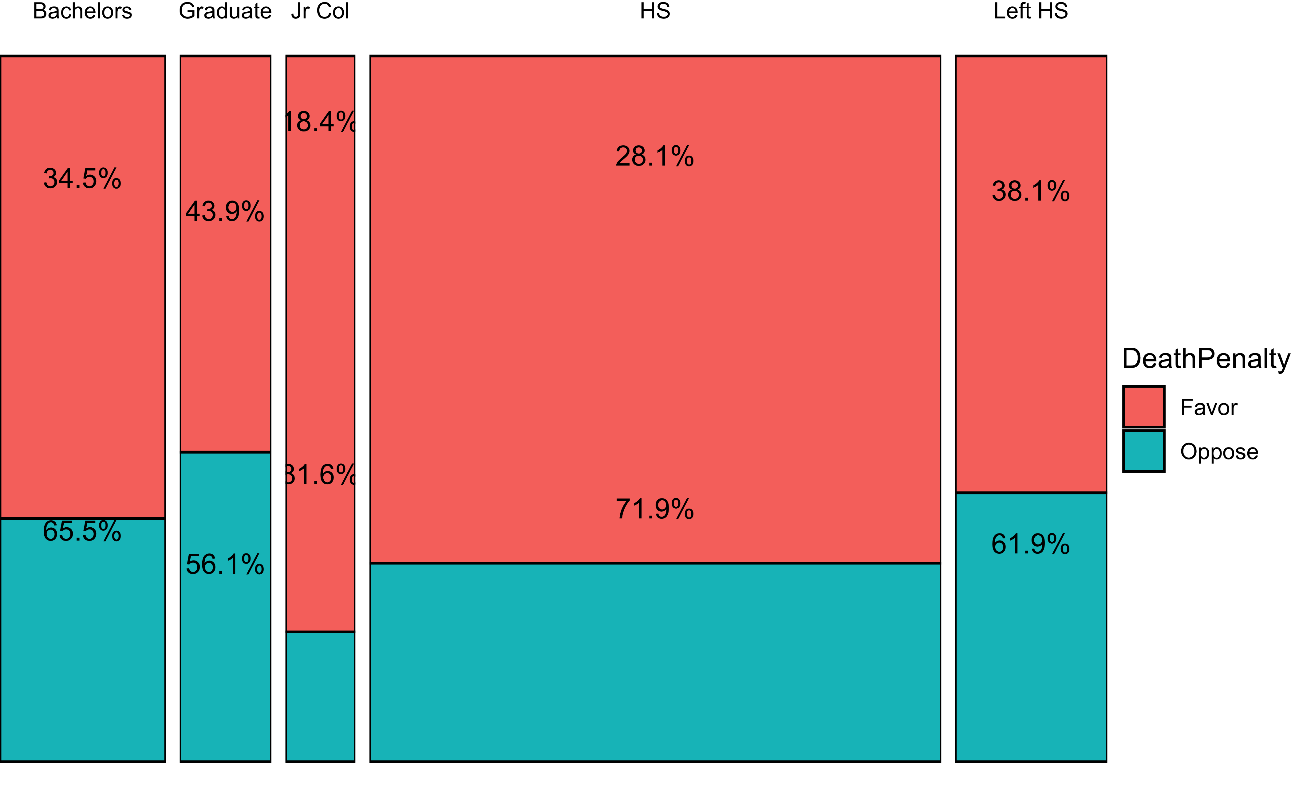
4.2 Using ggmosaic
# library(ggmosaic)

ggplot(data = gss2002) +
  geom_mosaic(aes(x = product(DeathPenalty, Education), fill = DeathPenalty))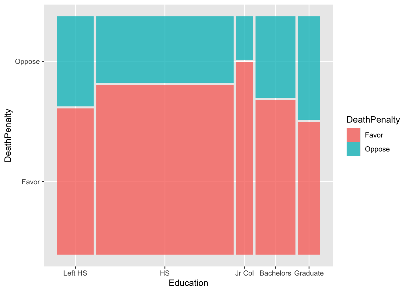
4.3 Observed Statistic: the X^2 metric
When there are multiple proportions involved, the X^2 test is what is used.
Let us now perform the base chisq test: We need a table and then the chisq test:
gss_table <- tally(DeathPenalty ~ Education, data = gss2002)
gss_table
Education
DeathPenalty Left HS HS Jr Col Bachelors Graduate
Favor 117 511 71 135 64
Oppose 72 200 16 71 50X.squared
23.45093 # Actual chi-square test
stats::chisq.test(tally(DeathPenalty ~ Education, data = gss2002))
    Pearson's Chi-squared test

data:  tally(DeathPenalty ~ Education, data = gss2002)
X-squared = 23.451, df = 4, p-value = 0.0001029
What would our Hypotheses be?
$$ H_0: Education Does Not affect Votes on Death Penalty\
H_a: Education affects Votes on Death Penalty
$$
We should now repeat the test with permutations on Education:
null_chisq <- do(10000) * chisq.test(tally(DeathPenalty ~ shuffle(Education), data = gss2002))

head(null_chisq)gf_histogram(~X.squared, data = null_chisq) %>%
gf_vline(xintercept = observedChi2, color = "red")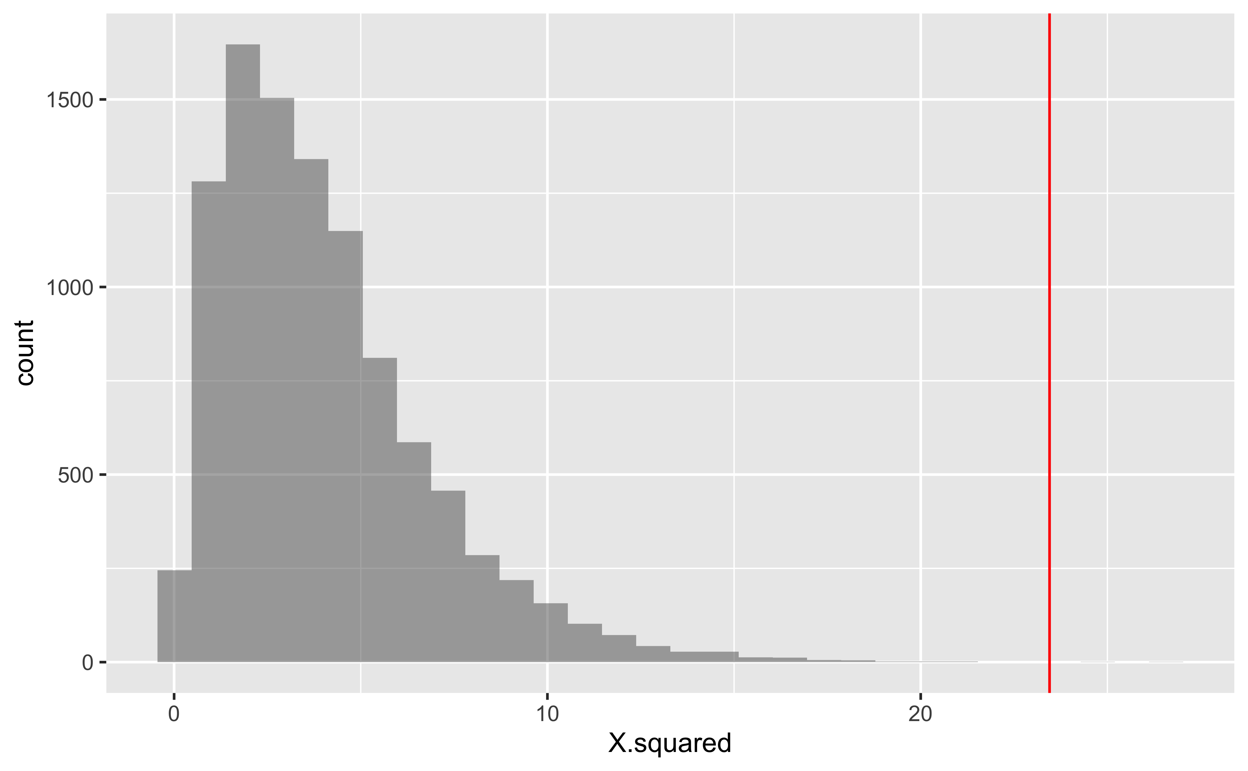
prop1(~ X.squared >= observedChi2, data = null_chisq) prop_TRUE
0.00019998 The p-value is well below our threshold of \(0.05%\), so we would conclude that Education has a significant effect on DeathPenalty opinion!
5 Conclusion
So, what do you think?