knitr::opts_chunk$set(echo = TRUE, message = TRUE, warning = TRUE, fig.align = "center")
library(tidyverse)
library(mosaic) # Our go-to package
library(infer) # An alternative package for inference using tidy data
library(broom) # Clean test results in tibble form
library(skimr) # data inspection

library(resampledata) # Datasets from Chihara and Hesterberg's book
library(openintro) # datasets
library(gt) # for tablesInference for Two Independent Means
1
1.1
flowchart TD
    A[Inference for Independent Means] -->|Check Assumptions| B[Normality: Shapiro-Wilk Test shapiro.test\n Variances: Fisher F-test var.test]
    B --> C{OK?}
    C -->|Yes, both\n Parametric| D[t.test]
    D <-->F[Linear Model\n Method]
    C -->|Yes, but not variance\n Parametric| W[t.test with\n Welch Correction]
    W<-->F
    C -->|No\n Non-Parametric| E[wilcox.test]
    E <--> G[Linear Model\n with\n Signed-Ranks]
    C -->|No\n Non-Parametric| P[Bootstrap\n or\n Permutation]
    P <--> Q[Linear Model\n with Signed-Rank\n with Permutation]
flowchart TD
A[Inference for Independent Means] -->|Check Assumptions| B[Normality: Shapiro-Wilk Test shapiro.test\n Variances: Fisher F-test var.test]
B --> C{OK?}
C -->|Yes, both\n Parametric| D[t.test]
D <-->F[Linear Model\n Method]
C -->|Yes, but not variance\n Parametric| W[t.test with\n Welch Correction]
W<-->F
C -->|No\n Non-Parametric| E[wilcox.test]
E <--> G[Linear Model\n with\n Signed-Ranks]
C -->|No\n Non-Parametric| P[Bootstrap\n or\n Permutation]
P <--> Q[Linear Model\n with Signed-Rank\n with Permutation]
2
NoteResearch Question
TBD
2.1
2.1.1 A.
Statistical tests for means usually require a couple of checks1 2:
- Are the data normally distributed?
- Are the data variances similar?:
Let us also complete a check for normality: the shapiro.wilk test checks whether a Quant variable is from a normal distribution; the NULL hypothesis is that the data are from a normal distribution.
2.1.2 B.
ImportantConditions:
- The two variables are not normally distributed.
- The two variances are also significantly different.
2.2
2.3
2.4
Type this in your console:
help(yrbss)Type help(wilcox.test) in your Console.
3
Every two years, the Centers for Disease Control and Prevention in the USA conduct the Youth Risk Behavior Surveillance System (YRBSS) survey, where it takes data from highschoolers (9th through 12th grade), to analyze health patterns. We will work with a selected group of variables from a random sample of observations during one of the years the YRBSS was conducted.
3.1
We have 13K data entries, and with 13 different variables, some Qual and some Quant. Many entries are missing too, typical of real-world data and something we will have to account for in our computations. The meaning of each variable can be found by bringing up the help file.
In this tutorial, our research question is:
NoteResearch Question
Does weight of highschoolers in this dataset vary with gender?
3.2
First, histograms and densities of the variable we are interested in:
yrbss_select_gender <- yrbss %>%
  select(weight, gender, physically_active_7d) %>%
  drop_na(weight) # Sadly dropping off NA data

yrbss_select_gender %>%
  gf_density(~weight,
    fill = ~gender,
    alpha = 0.5,
    title = "Highschoolers' Weights by Gender"
  ) %>%
  gf_theme(theme_classic())
yrbss_select_gender %>%
  gf_boxplot(weight ~ gender,
    fill = ~gender,
    alpha = 0.5,
    title = "Highschoolers' Weights by Gender"
  ) %>%
  gf_theme(theme_classic())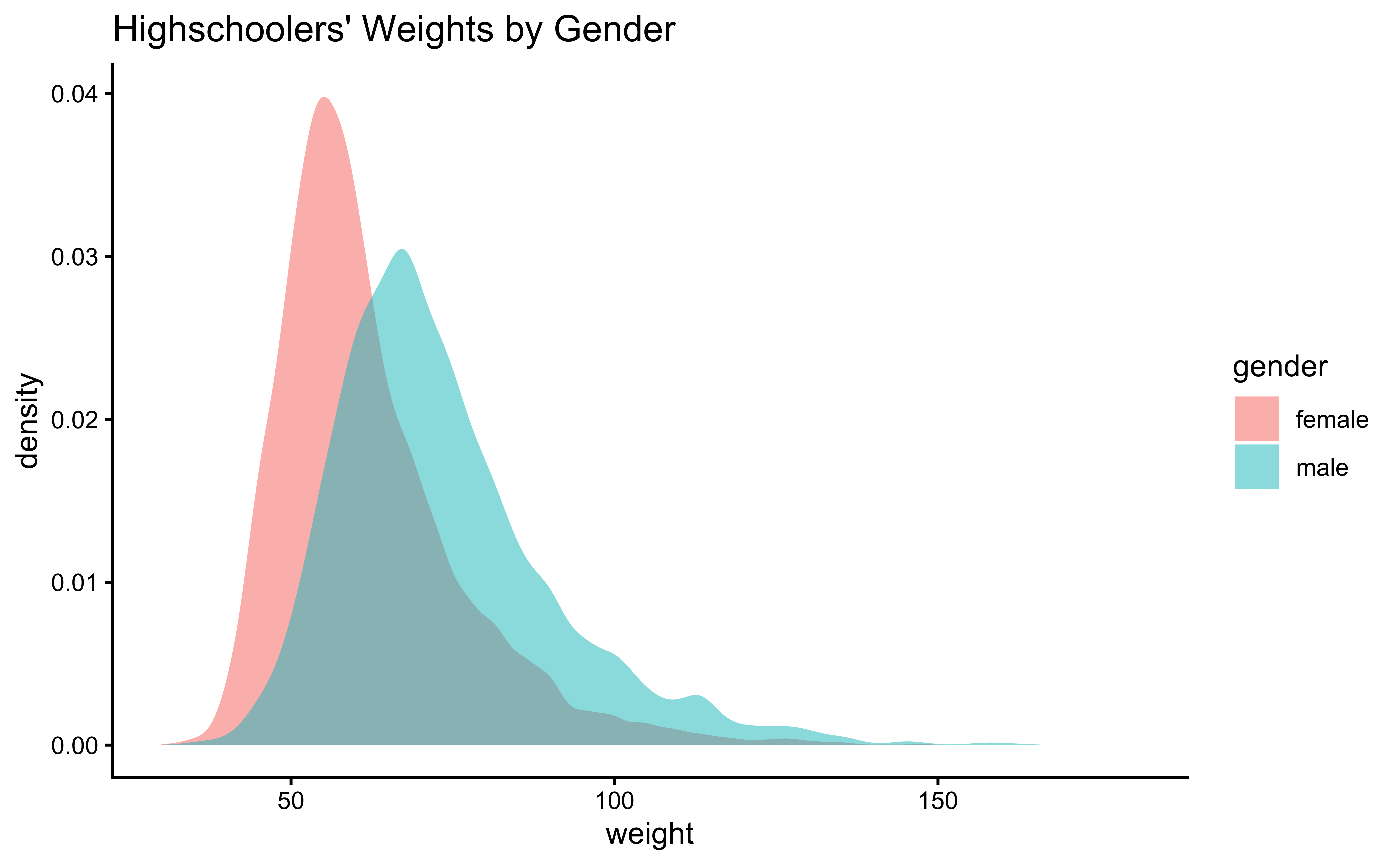
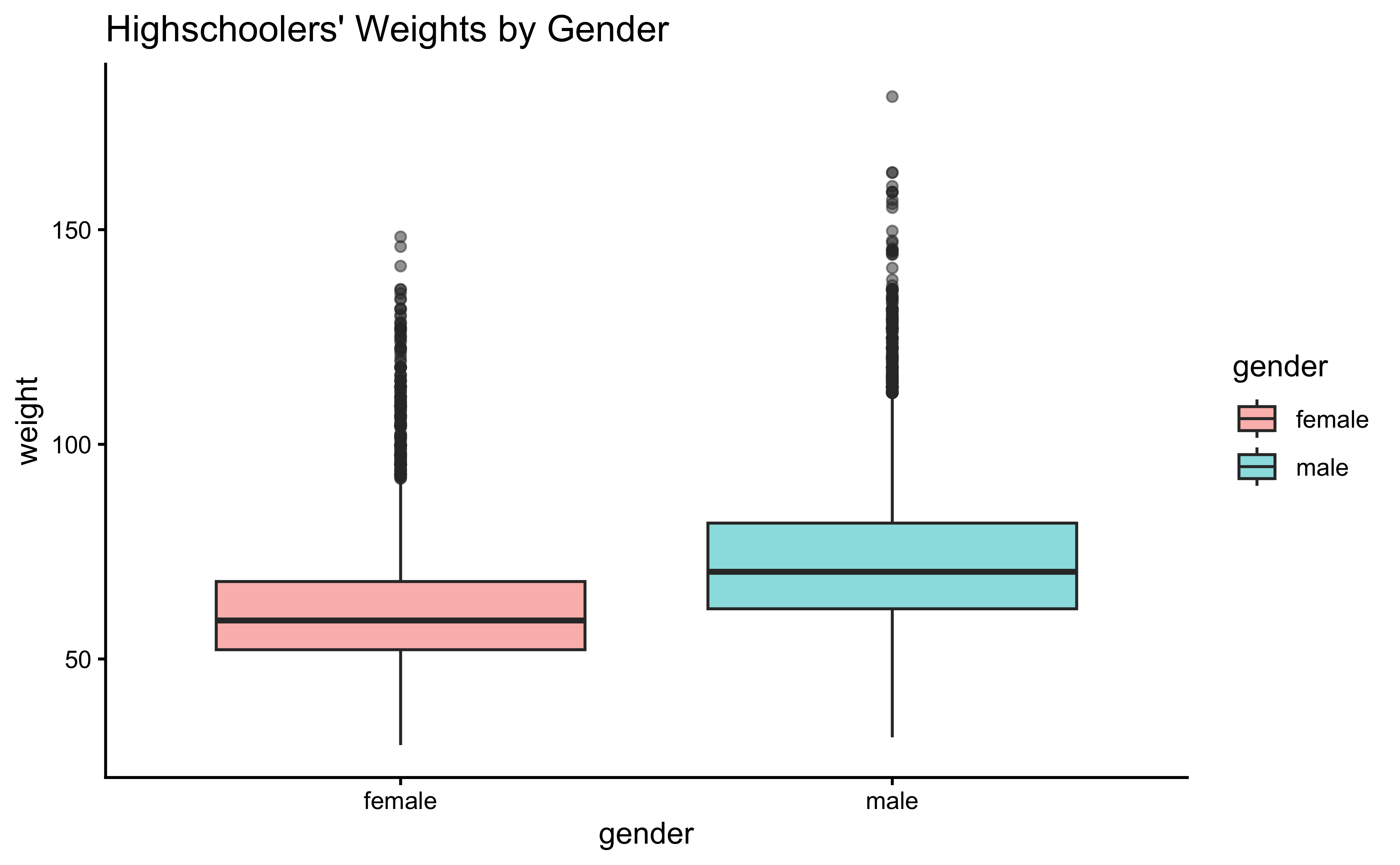
Overlapped Distribution plot shows some difference in the means; and the Boxplots show visible difference in the medians.
As stated before, statistical tests for means usually require a couple of checks:
- Are the data normally distributed?
- Are the data variances similar?
Let us also complete a visual check for normality,with plots since we cannot do a shapiro.test:
NoteShapiro-Wilks Test
The longest data it can take (in R) is 5000. Since our data is longer, we will cannot use this procedure and have to resort to visual means.
male_student_weights <- yrbss_select_gender %>%
  filter(gender == "male") %>%
  select(weight)
female_student_weights <- yrbss_select_gender %>%
  filter(gender == "female") %>%
  select(weight)
# shapiro.test(male_student_weights$weight)
# shapiro.test(female_student_weights$weight)

yrbss_select_gender %>%
  gf_density(~weight,
    fill = ~gender,
    alpha = 0.5,
    title = "Highschoolers' Weights by Gender"
  ) %>%
  gf_facet_grid(~gender) %>%
  gf_fitdistr(dist = "dnorm") %>%
  gf_theme(theme_classic())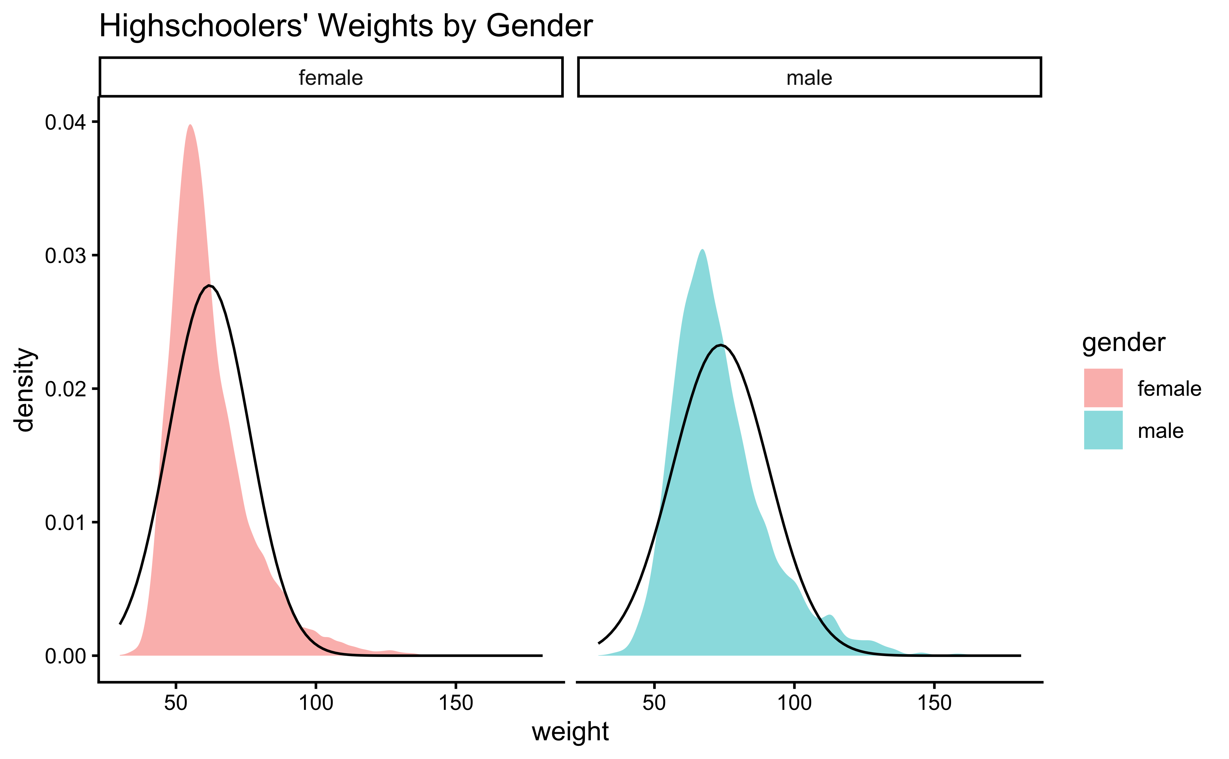
Distributions are not too close to normal…perhaps a hint of a rightward skew, suggesting that there are some obese students.
We can plot Q-Q plots3 for both variables, and also compare both data with normally-distributed data generated with the same means and standard deviations:
yrbss_select_gender %>%
  gf_qq(~ weight | gender) %>%
  gf_qqline(ylab = "scores") %>%
  gf_theme(theme_classic())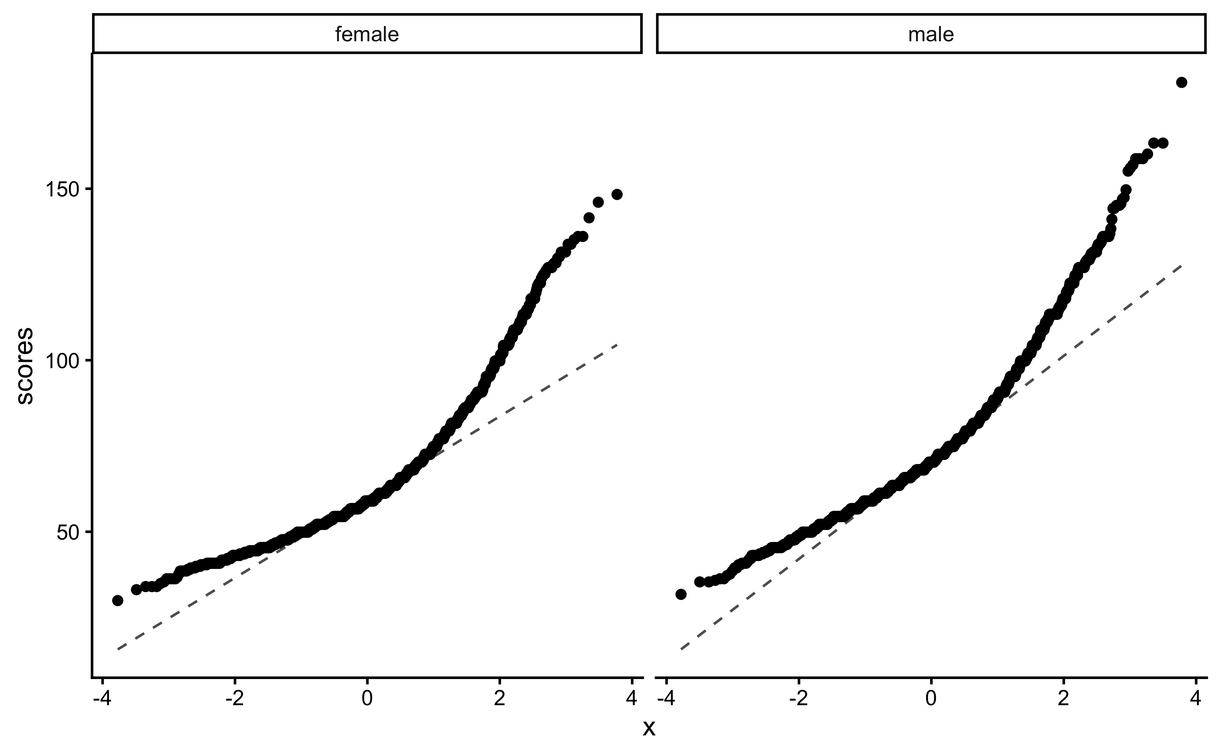
No real evidence (visually) of the variables being normally distributed.
Let us check if the two variables have similar variances: the var.test does this for us, with a NULL hypothesis that the variances are not significantly different:
The p.value being so small, we are able to reject the NULL Hypothesis that the variances of weight are nearly equal across the two exercise regimes.
ImportantConditions
- The two variables are not normally distributed.
- The two variances are also significantly different.
This means that the parametric t.test must be eschewed in favour of the non-parametric wilcox.test. We will use that, and also attempt linear models with rank data, and a final permutation test.
3.3
Based on the graphs, how would we formulate our Hypothesis? We wish to infer whether there is difference in mean weight across gender. So accordingly:
\[ H_0: \mu_{male} = \mu_{female}\\ \\\ H_a: \mu_{male} \ne \mu_{female}\ \]
3.4
What would be the test statistic we would use? The difference in means. Is the observed difference in the means between the two groups of scores non-zero? We use the diffmean function, from mosaic:
obs_diff_gender <- diffmean(weight ~ gender, data = yrbss_select_gender)

obs_diff_gender
diffmean
11.70089
3.5
Since the data variables do not satisfy the assumption of being normally distributed, and the variances are significantly different, we use the classical wilcox.test, which implements what we need here: the Mann-Whitney U test:4
The Mann-Whitney test as a test of mean ranks. It first ranks all your values from high to low, computes the mean rank in each group, and then computes the probability that random shuffling of those values between two groups would end up with the mean ranks as far apart as, or further apart, than you observed. No assumptions about distributions are needed so far. (emphasis mine)
We will use the mosaic variant). Our model would be:
\[ mean(rank(Weight_{male})) - mean(rank(Weight_{female})) = \beta_0 \\\ H_0: \beta_0 = 0;\\ \\\ H_a: \beta_0 \ne 0 \]
wilcox.test(weight ~ gender,
  data = yrbss_select_gender,
  conf.int = TRUE,
  conf.level = 0.95
) %>%
  broom::tidy()
The p.value is negligible and we are able to reject the NULL hypothesis that the means are equal.
We can apply the linear-model-as-inference interpretation to the ranked data data to implement the non-parametric test as a Linear Model:
\[ lm(rank(weight) \sim gender) = \beta_0 + \beta_1 * gender \\ H_0: \beta_1 = 0\\ \\\ H_a: \beta_1 \ne 0\\ \]
TipDummy Variables in
lm
Note how the Qual variable was used here in Linear Regression! The gender variable was treated as a binary “dummy” variable5.
We saw from the diagram created by Allen Downey that there is only one test6! We will now use this philosophy to develop a technique that allows us to mechanize several Statistical Models in that way, with nearly identical code. For the specific data at hand, we need to shuffle the records between Semifinal and Final on a per Swimmer basis and take the test statistic (difference between the two swim records for each swimmer). Another way to look at this is to take the differences between Semifinal and Final scores and shuffle the differences to either polarity. We will follow this method in the code below:
null_dist_weight <-
  do(9999) * diffmean(data = yrbss_select_gender, weight ~ shuffle(gender))
null_dist_weight
gf_histogram(data = null_dist_weight, ~diffmean, bins = 25) %>%
  gf_vline(xintercept = obs_diff_gender, colour = "red") %>%
  gf_theme(theme_classic())
gf_ecdf(data = null_dist_weight, ~diffmean) %>%
  gf_vline(xintercept = obs_diff_gender, colour = "red") %>%
  gf_theme(theme_classic())
prop1(~ diffmean <= obs_diff_gender, data = null_dist_weight)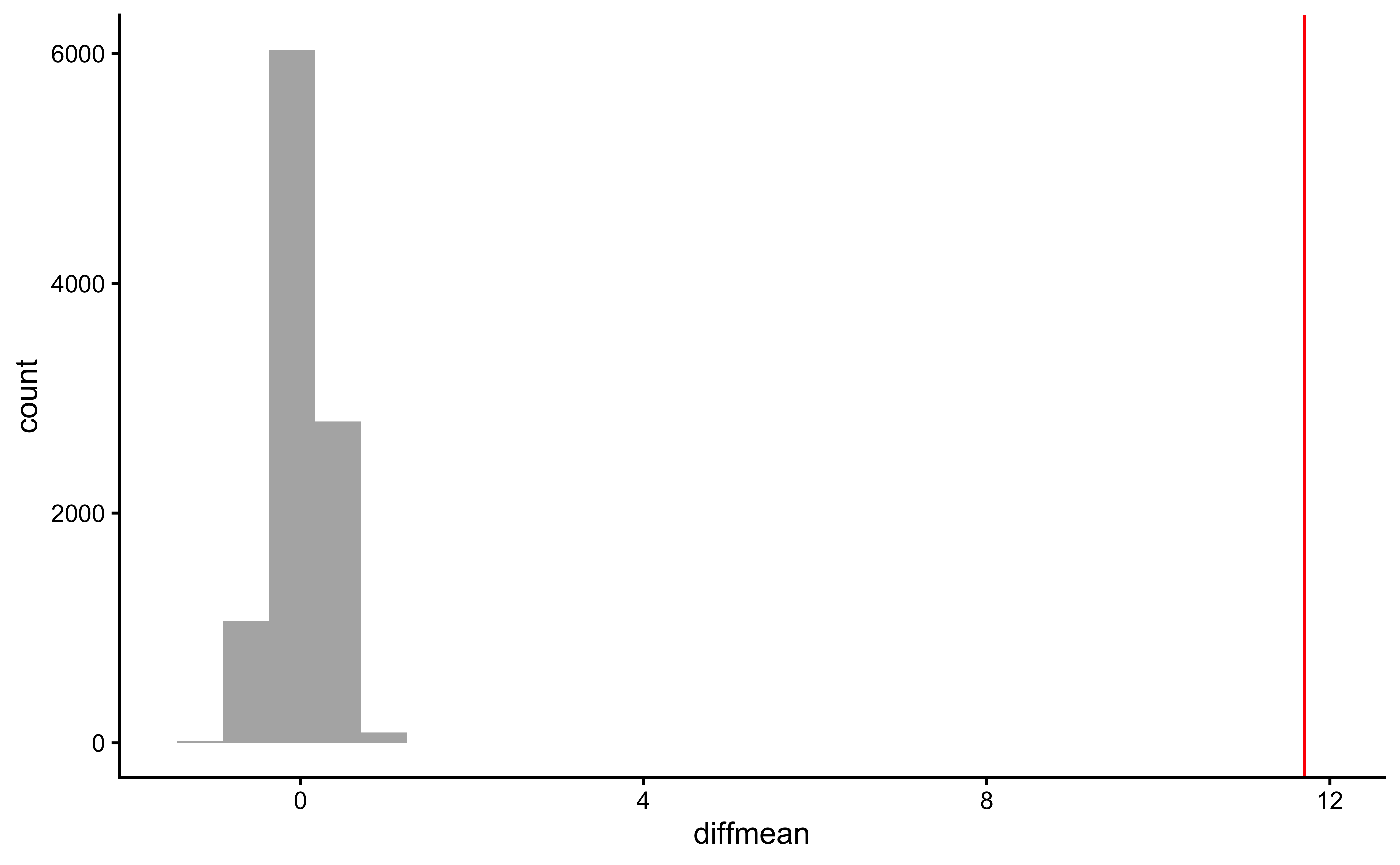
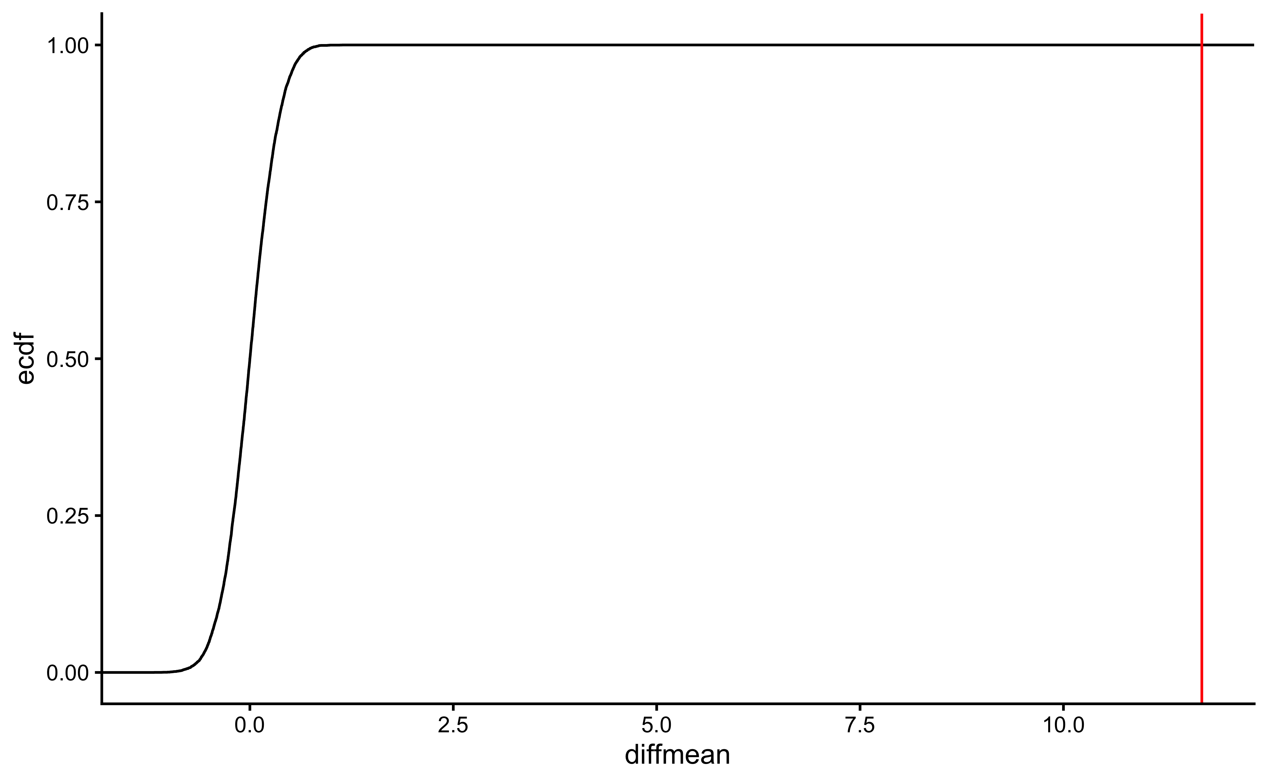
prop_TRUE
        1
Clearly the observed_diff_weight is much beyond anything we can generate with permutations with gender! And hence there is a significant difference in weights across gender!
We can put all the test results together to get a few more insights about the tests:
wilcox.test(weight ~ gender,
  data = yrbss_select_gender,
  conf.int = TRUE,
  conf.level = 0.95
) %>%
  broom::tidy() %>%
  gt() %>%
  tab_style(
    style = list(cell_fill(color = "cyan"), cell_text(weight = "bold")),
    locations = cells_body(columns = p.value)
  ) %>%
  tab_header(title = "wilcox.test")

lm(rank(weight) ~ gender,
  data = yrbss_select_gender
) %>%
  broom::tidy(
    conf.int = TRUE,
    conf.level = 0.95
  ) %>%
  gt() %>%
  tab_style(
    style = list(cell_fill(color = "cyan"), cell_text(weight = "bold")),
    locations = cells_body(columns = p.value)
  ) %>%
tab_header(title = "Linear Model with Ranked Data")| wilcox.test | ||||||
| estimate | statistic | p.value | conf.low | conf.high | method | alternative |
|---|---|---|---|---|---|---|
| -11.33999 | 10808212 | 0 | -11.34003 | -10.87994 | Wilcoxon rank sum test with continuity correction | two.sided |
| Linear Model with Ranked Data | ||||||
| term | estimate | std.error | statistic | p.value | conf.low | conf.high |
|---|---|---|---|---|---|---|
| (Intercept) | 4836.157 | 42.52745 | 113.71848 | 0 | 4752.797 | 4919.517 |
| gendermale | 2851.246 | 59.55633 | 47.87478 | 0 | 2734.507 | 2967.986 |
The wilcox.test and the linear model with rank data offer the same results. This is of course not surprising!
4
Next, consider the possible relationship between a highschooler’s weight and their physical activity.
First, let’s create a new variable physical_3plus, which will be coded as either “yes” if the student is physically active for at least 3 days a week, and “no” if not. Recall that we have several missing data in that column, so we will (sadly) drop these before generating the new variable:
yrbss_select_phy <- yrbss %>%
  drop_na(physically_active_7d, weight) %>%
  mutate(
    physical_3plus = if_else(physically_active_7d >= 3, "yes", "no"),
    physical_3plus = factor(physical_3plus,
      labels = c("yes", "no"),
      levels = c("yes", "no")
    )
  ) %>%
  select(weight, physical_3plus)

# Let us check
yrbss_select_phy %>% count(physical_3plus)
NoteResearch Question
Does weight vary based on whether students exercise on more or less than 3 days a week? (physically_active_7d >= 3 days)
4.1
We can make distribution plots for weight by physical_3plus:
gf_boxplot(weight ~ physical_3plus,
  fill = ~physical_3plus,
  data = yrbss_select_phy, xlab = "Days of Exercise >=3 "
) %>%
  gf_theme(theme_classic())
gf_density(~weight,
  fill = ~physical_3plus,
  data = yrbss_select_phy
) %>%
  gf_theme(theme_classic())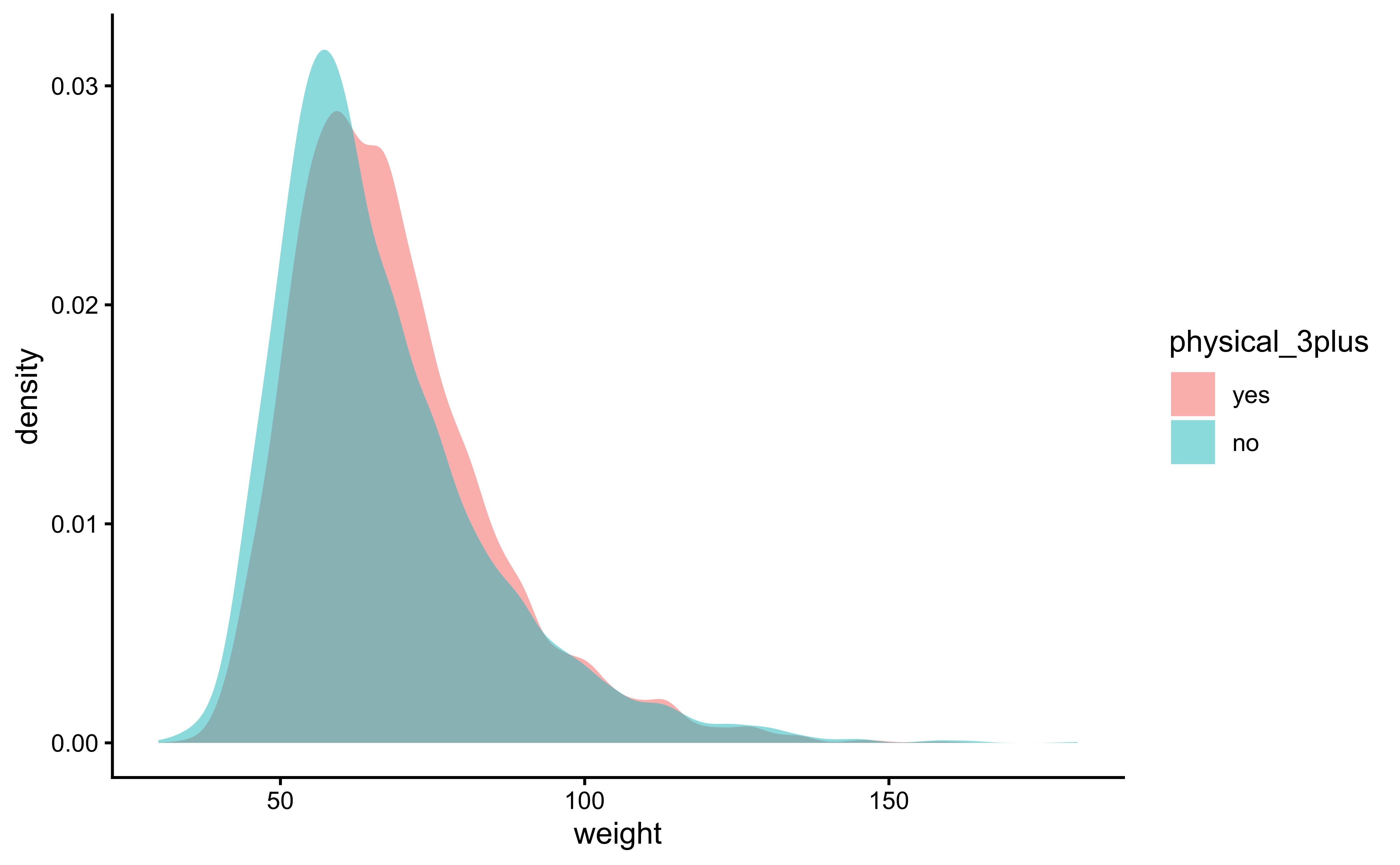
The box plots show how the medians of the two distributions compare, but we can also compare the means of the distributions using the following to first group the data by the physical_3plus variable, and then calculate the mean weight in these groups using the mean function while ignoring missing values by setting the na.rm argument to TRUE.
There is an observed difference, but is this difference large enough to deem it “statistically significant”? In order to answer this question we will conduct a hypothesis test. But before that a few more checks on the data:
As stated before, statistical tests for means usually require a couple of checks:
- Are the data normally distributed?
- Are the data variances similar?
Let us also complete a visual check for normality,with plots since we cannot do a shapiro.test:
yrbss_select_phy %>%
  gf_density(~weight,
    fill = ~physical_3plus,
    alpha = 0.5,
    title = "Highschoolers' Weights by Exercise Frequency"
  ) %>%
  gf_facet_grid(~physical_3plus) %>%
  gf_fitdistr(dist = "dnorm") %>%
  gf_theme(theme_classic())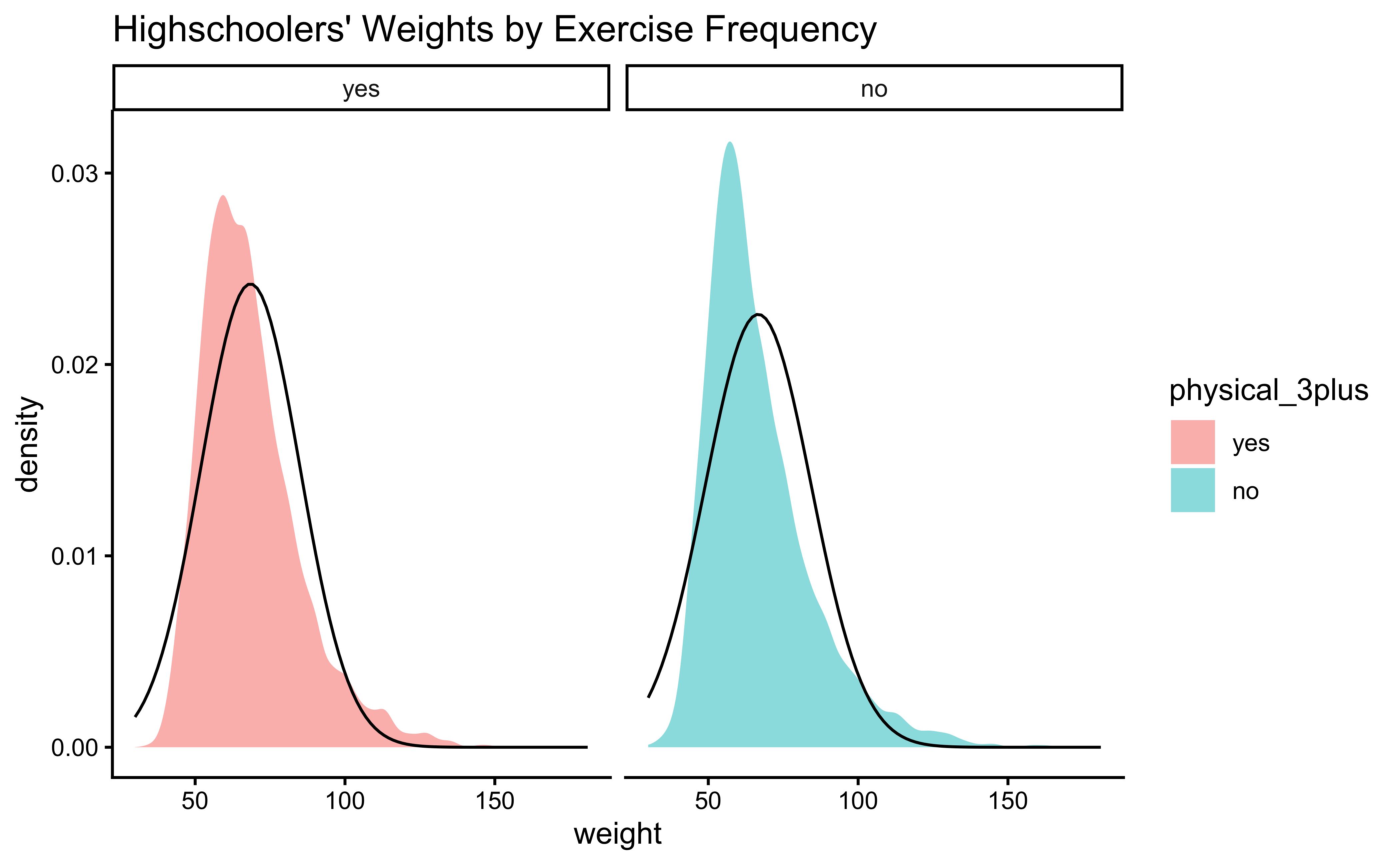
Again, not normally distributed…
We can plot Q-Q plots for both variables, and also compare both data with normally-distributed data generated with the same means and standard deviations:
yrbss_select_phy %>%
  gf_qq(~ weight | physical_3plus, color = ~physical_3plus) %>%
  gf_qqline(ylab = "Weight") %>%
  gf_theme(theme_classic())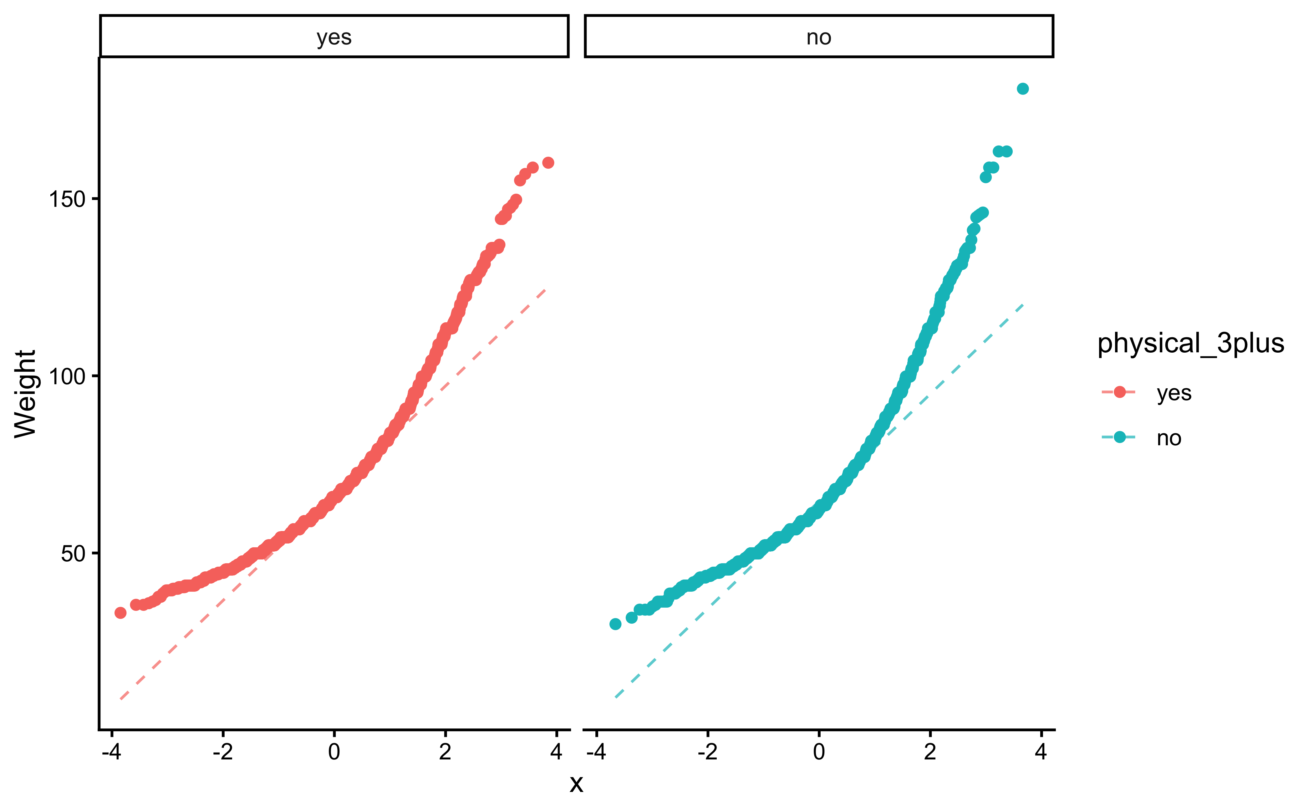
The QQ-plots confirm that he tow data variables are not normally distributed.
Let us check if the two variables have similar variances: the var.test does this for us, with a NULL hypothesis that the variances are not significantly different:
[1] 1.054398The p.value states the probability of the data being what it is, assuming the NULL hypothesis that variances were similar. It being so small, we are able to reject this NULL Hypothesis that the variances of weight are nearly equal across the two exercise frequencies. (Compare the statistic in the var.test with the critical F-value)
ImportantConditions
- The two variables are not normally distributed.
- The two variances are also significantly different.
Hence we will have to use non-parametric tests to infer if the means are similar.
4.2
Based on the graphs, how would we formulate our Hypothesis? We wish to infer whether there is difference in mean weight across physical_3plus. So accordingly:
\[ H_0: \mu_{physical-3plus-Yes} = \mu_{physical-3plus-No}\\ \\\ H_a: \mu_{physical-3plus-Yes} \ne \mu_{physical-3plus-No}\\ \]
4.3
Statistic
What would be the test statistic we would use? The difference in means. Is the observed difference in the means between the two groups of scores non-zero? We use the diffmean function, from mosaic:
obs_diff_phy <- diffmean(weight ~ physical_3plus, data = yrbss_select_phy)

obs_diff_phy
diffmean
-1.774584 Well, the variables are not normally distributed, and the variances are significantly different so a standard t.test is not advised. We can still try:
The p.value is \(8.9e-08\) ! And the Confidence Interval is clear of \(0\). So the t.test gives us good reason to reject the Null Hypothesis that the means are similar. But can we really believe this, given the non-normality of data?
However, we have seen that the data variables are not normally distributed. So a Wilcoxon Test, using signed-ranks, is indicated: (recall the model!)
# For stability reasons, it may be advisable to use rounded data or to set digits.rank = 7, say,
# such that determination of ties does not depend on very small numeric differences (see the example).
wilcox.test(weight ~ physical_3plus,
conf.int = TRUE,
conf.level = 0.95,
data = yrbss_select_phy
) %>%
broom::tidy()The nonparametric wilcox.test also suggests that the means for weight across physical_3plus are significantly different.
4.3.1 Using the Linear Model Interpretation
We can apply the linear-model-as-inference interpretation to the ranked data data to implement the non-parametric test as a Linear Model:
\[ lm(rank(weight) \sim physical.3plus) = \beta_0 + \beta_1 \times physical.3plus \\ H_0: \beta_1 = 0\\ \\\ H_a: \beta_1 \ne 0\\ \]
Here too, the linear model using rank data arrives at a conclusion similar to that of the Mann-Whitney U test.
4.3.2 Using Permutation Tests
We will do this in two ways, just for fun: one using mosaic and the other using infer.
But first, we need to initialize the test, which we will save as obs_diff.
 diffmean
-1.774584 diffmean
-1.774584
Important
Note that obs_diff_infer is a 1 X 1 dataframe; obs_diff_mosaic is a scalar!!
We already have the observed difference, obs_diff_mosaic. Now we generate the null distribution using permutation, with mosaic:
We can also generate the histogram of the null distribution, compare that with the observed diffrence and compute the p-value and confidence intervals:
gf_histogram(~diffmean, data = null_dist_mosaic) %>%
  gf_vline(xintercept = obs_diff_mosaic, colour = "red")
`stat_bin()` using `bins = 30`. Pick better value `binwidth`.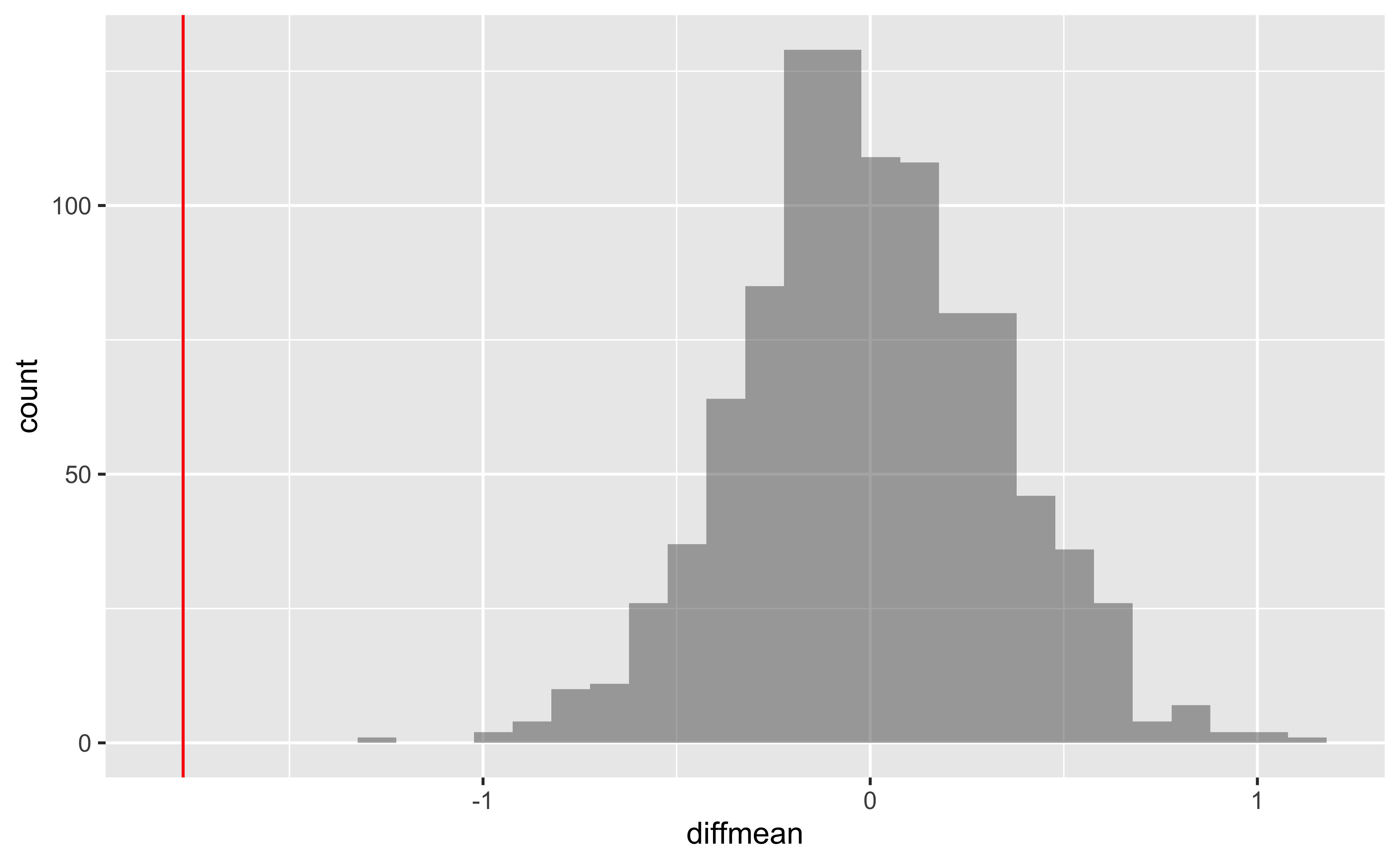
# p-value
prop(~ diffmean != obs_diff_mosaic, data = null_dist_mosaic)
prop_TRUE
1 # Confidence Intervals for p = 0.95
mosaic::cdata(~diffmean, p = 0.95, data = null_dist_mosaic)4.4 Your Turn
Calculate a 95% confidence interval for the average height in meters (
height) and interpret it in context.Calculate a new confidence interval for the same parameter at the 90% confidence level. Comment on the width of this interval versus the one obtained in the previous exercise.
Conduct a hypothesis test evaluating whether the average height is different for those who exercise at least three times a week and those who don’t.
Now, a non-inference task: Determine the number of different options there are in the dataset for the
hours_tv_per_school_daythere are.Come up with a research question evaluating the relationship between height or weight and sleep. Formulate the question in a way that it can be answered using a hypothesis test and/or a confidence interval. Report the statistical results, and also provide an explanation in plain language. Be sure to check all assumptions, state your \(\alpha\) level, and conclude in context.
Footnotes
https://stats.stackexchange.com/questions/2492/is-normality-testing-essentially-useless↩︎
https://www.allendowney.com/blog/2023/01/28/never-test-for-normality/↩︎
https://stats.stackexchange.com/questions/92374/testing-large-dataset-for-normality-how-and-is-it-reliable↩︎
https://allendowney.blogspot.com/2016/06/there-is-still-only-one-test.html↩︎