Correlation and Regression Explorations

Author

Arvind V

1 Packages

library(tidyverse)
library(mosaic)
library(broom)
library(ggformula)
ggplot2::theme_set(new = theme_classic())

Plot Fonts and Theme

Show the Code

library(systemfonts)
library(showtext)
library(tidyverse)
## Clean the slate
systemfonts::clear_local_fonts()
systemfonts::clear_registry()
##
showtext_opts(dpi = 96) # set DPI for showtext
sysfonts::font_add(
  family = "Alegreya",
  regular = "../../../../../../../fonts/Alegreya-Regular.ttf",
  bold = "../../../../../../../fonts/Alegreya-Bold.ttf",
  italic = "../../../../../../../fonts/Alegreya-Italic.ttf",
  bolditalic = "../../../../../../../fonts/Alegreya-BoldItalic.ttf"
)

sysfonts::font_add(
  family = "Roboto Condensed",
  regular = "../../../../../../../fonts/RobotoCondensed-Regular.ttf",
  bold = "../../../../../../../fonts/RobotoCondensed-Bold.ttf",
  italic = "../../../../../../../fonts/RobotoCondensed-Italic.ttf",
  bolditalic = "../../../../../../../fonts/RobotoCondensed-BoldItalic.ttf"
)
showtext_auto(enable = TRUE) # enable showtext
##
theme_custom <- function() {
  font <- "Alegreya" # assign font family up front
  "%+replace%" <- ggplot2::"%+replace%" # nolint

  ggplot2::theme_classic(base_size = 14, base_family = font) %+replace% # replace elements we want to change

    theme(
      text = element_text(family = font), # set base font family

      # text elements
      plot.title = element_text( # title
        family = font, # set font family
        size = 24, # set font size
        face = "bold", # bold typeface
        hjust = 0, # left align
        margin = margin(t = 5, r = 0, b = 5, l = 0)
      ), # margin
      plot.title.position = "plot",
      plot.subtitle = element_text( # subtitle
        family = font, # font family
        size = 14, # font size
        hjust = 0, # left align
        margin = margin(t = 5, r = 0, b = 10, l = 0)
      ), # margin

      plot.caption = element_text( # caption
        family = font, # font family
        size = 9, # font size
        hjust = 1
      ), # right align

      plot.caption.position = "plot", # right align

      axis.title = element_text( # axis titles
        family = "Roboto Condensed", # font family
        size = 12
      ), # font size

      axis.text = element_text( # axis text
        family = "Roboto Condensed", # font family
        size = 9
      ), # font size

      axis.text.x = element_text( # margin for axis text
        margin = margin(5, b = 10)
      )

      # since the legend often requires manual tweaking
      # based on plot content, don't define it here
    )
}

## Use available fonts in ggplot text geoms too!
ggplot2::update_geom_defaults(geom = "text", new = list(
  family = "Roboto Condensed",
  face = "plain",
  size = 3.5,
  color = "#2b2b2b"
))

## Set the theme
ggplot2::theme_set(new = theme_custom())

2 Intro

I will work through and “unify” at least two things:

Hadley Wickham’s chapter on modelling and his analysis of the linear model for the diamonds dataset
The diagnostic aspects of Linear Regression as detailed in Crawley’s book

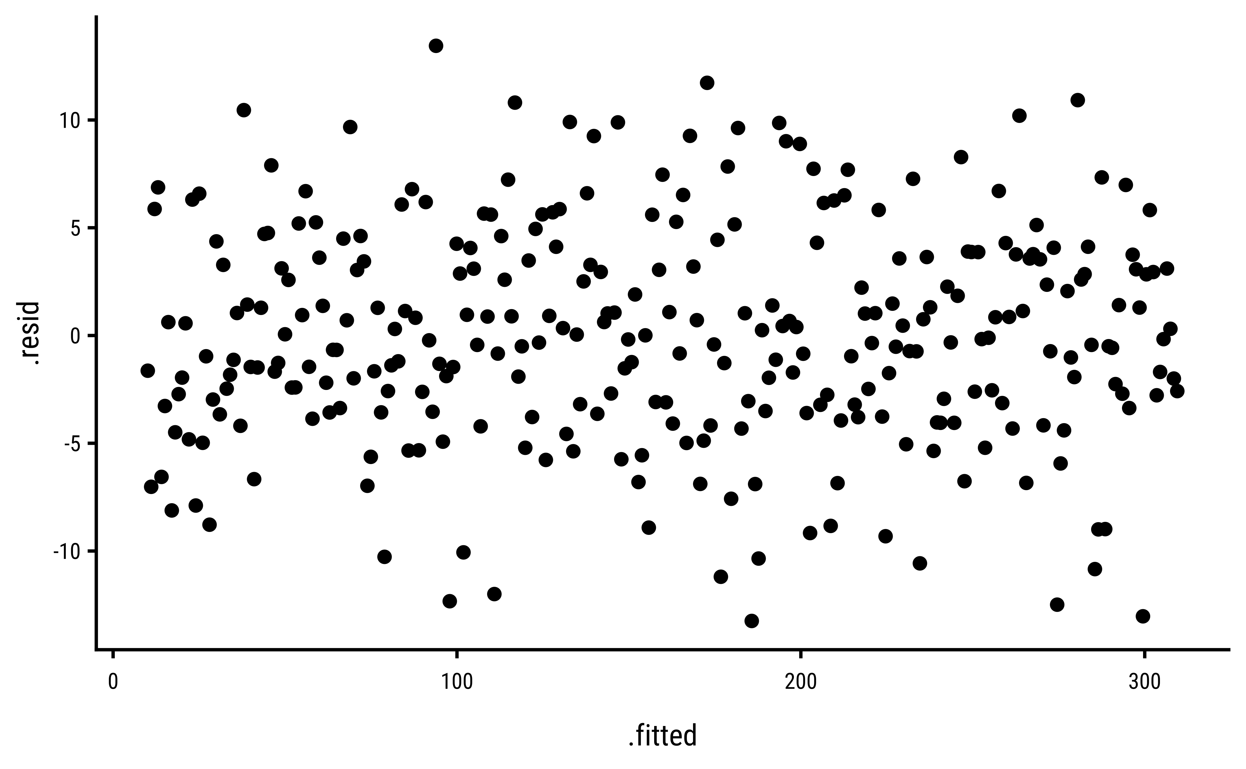
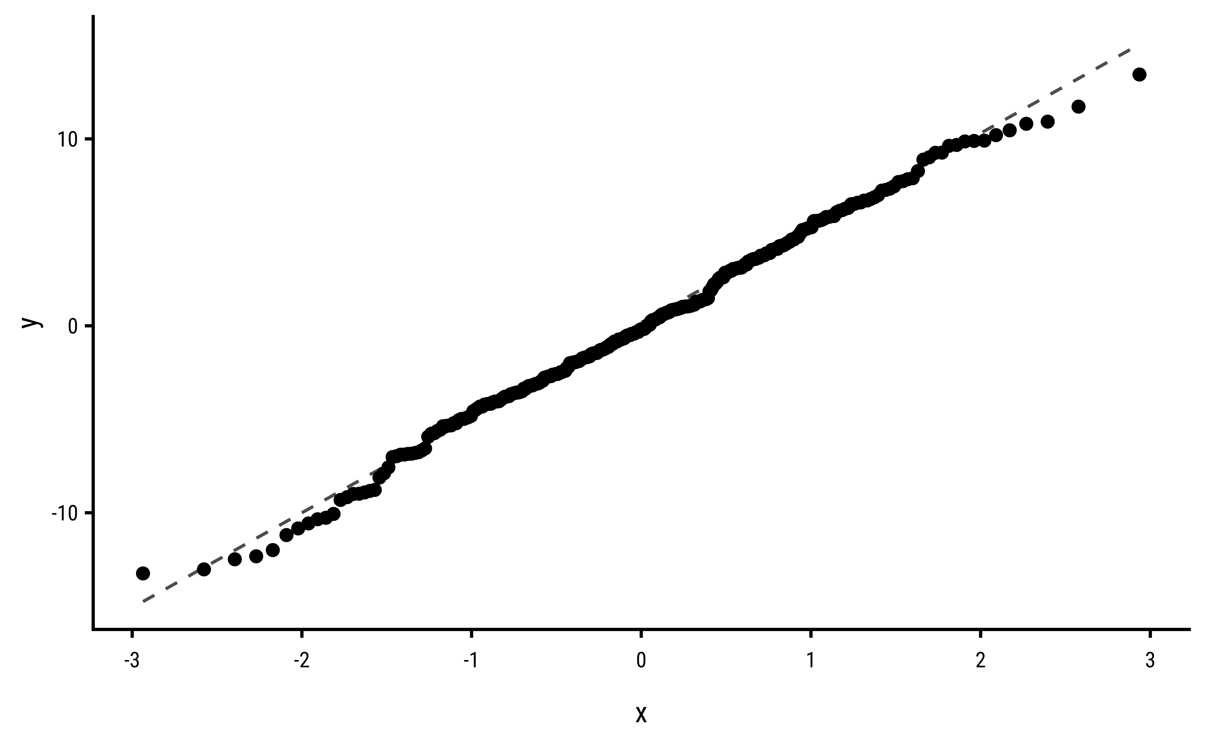
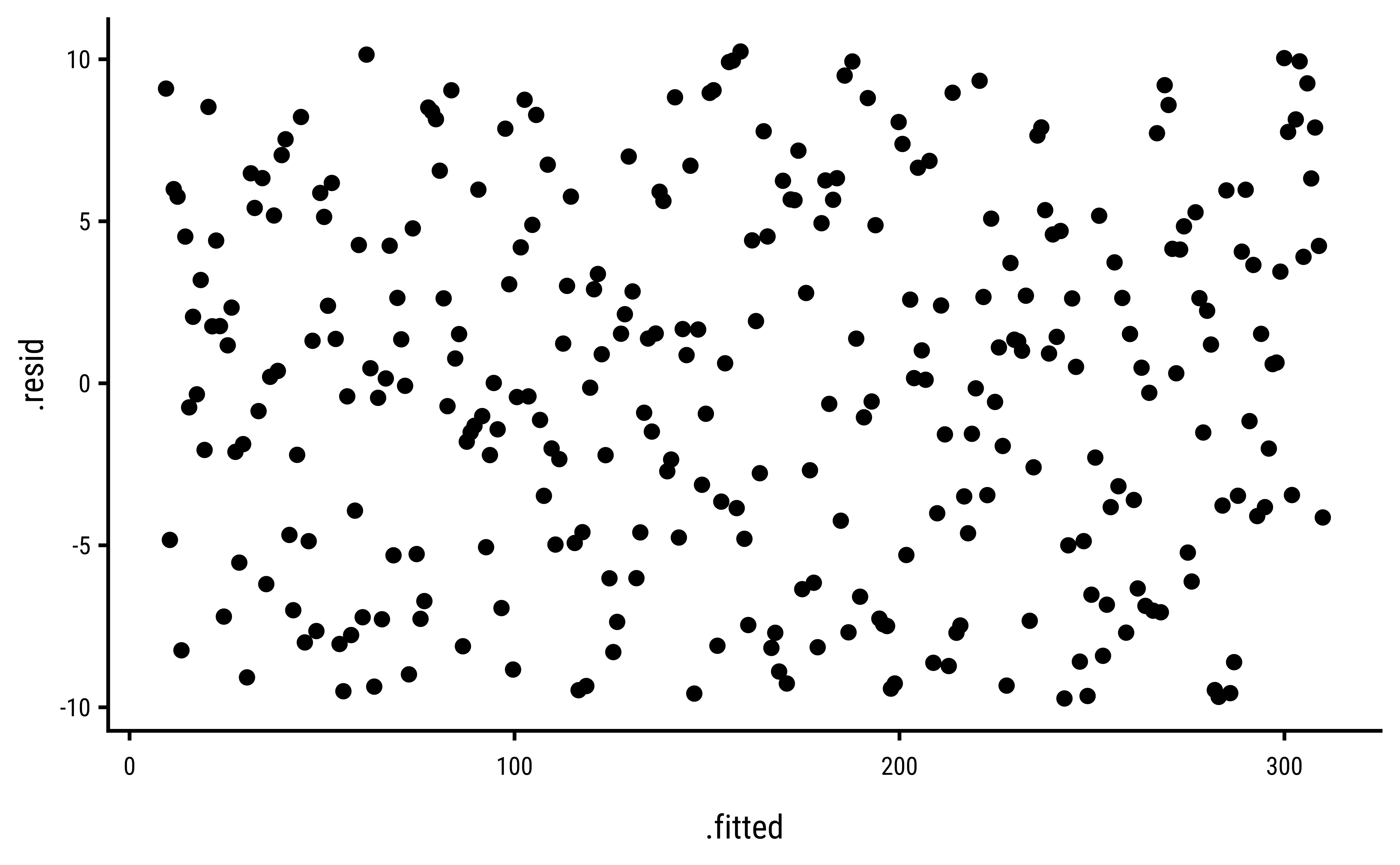
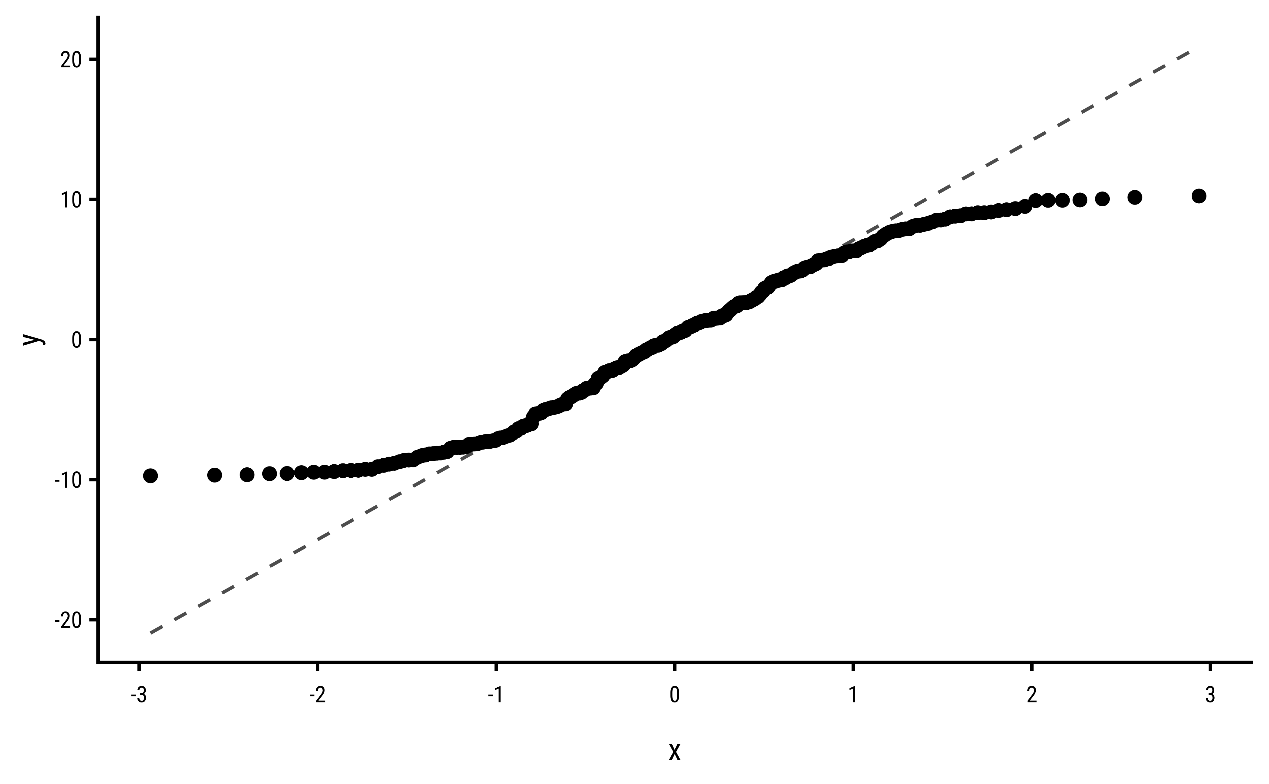
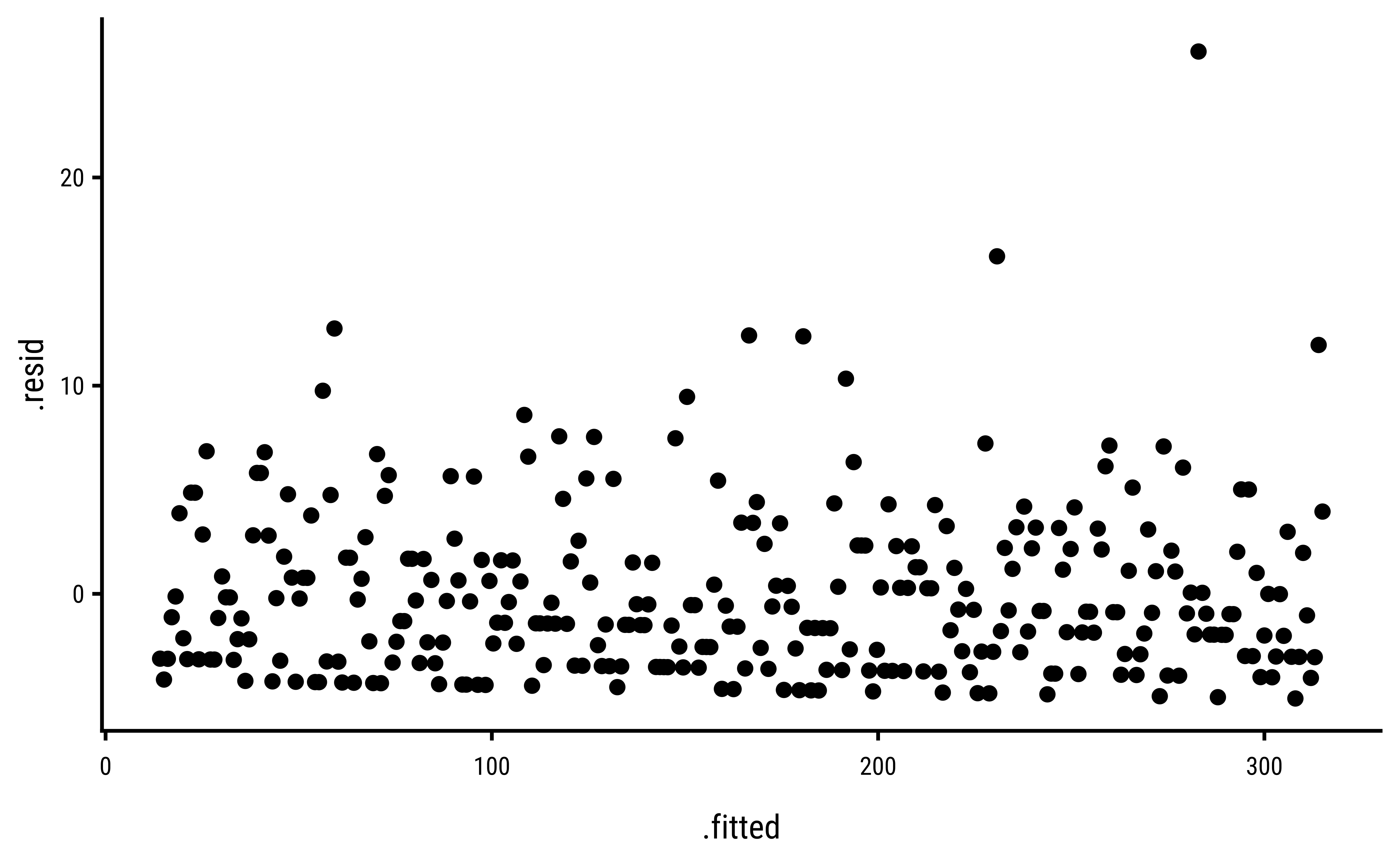
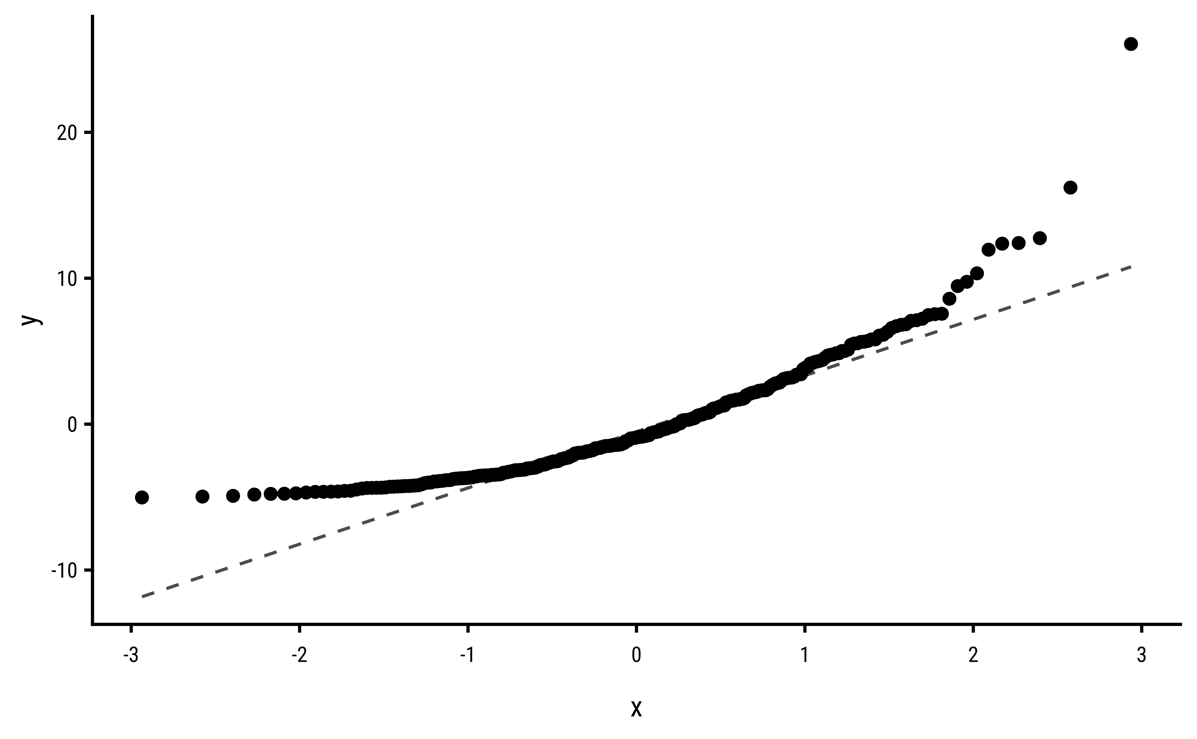
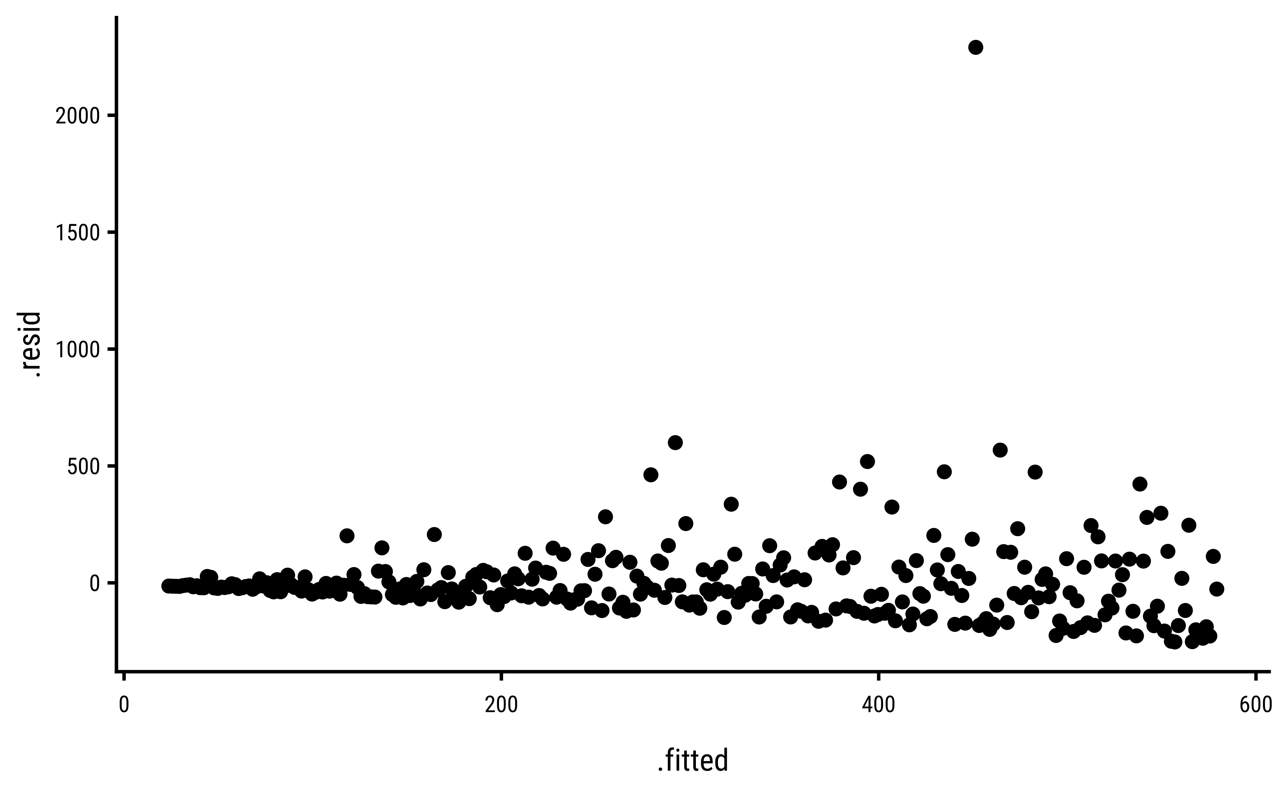
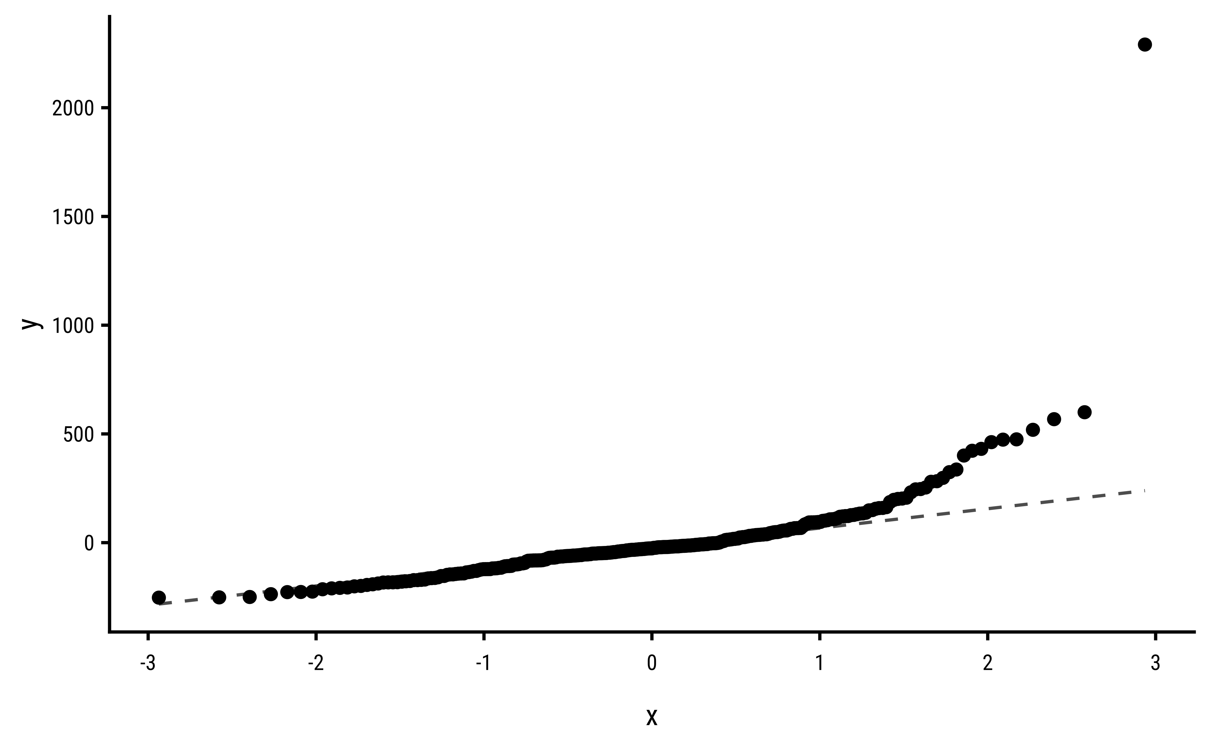
3 Explorations into Diagnostic Plots

Let us create dependent y* variables with different sorts of errors:

x <- 0:300
en <- rnorm(301, mean = 0, sd = 5)
eu <- (runif(n = 301) - 0.5) * 20
eb <- rnbinom(n = 301, prob = 0.3, size = 2)
eg <- rgamma(n = 301, shape = 1, rate = 1 / x)
yn <- x + 10 + en
yu <- x + 10 + eu
yb <- x + 10 + eb
yg <- x + 10 + eg
data <- tibble(x, yn, yu, yb, yg)
data

3.1 Normal Errors

lm_norm_aug <- lm(yn ~ x, data = data) %>%
  augment()
lm_norm_aug %>% gf_point(.resid ~ .fitted)

lm_norm_aug %>%
  gf_qq(~.resid) %>%
  gf_qqline()

3.2 Uniform Errors

lm_unif_aug <- lm(yu ~ x, data = data) %>%
  augment()
lm_unif_aug %>% gf_point(.resid ~ .fitted)

lm_unif_aug %>%
  gf_qq(~.resid, distribution = stats::qnorm) %>%
  gf_qqline()

3.3 Negative Binom Errors

lm_nbinom_aug <- lm(yb ~ x, data = data) %>%
  augment()
lm_nbinom_aug %>% gf_point(.resid ~ .fitted)

lm_nbinom_aug %>%
  gf_qq(~.resid, distribution = stats::qnorm) %>%
  gf_qqline()

3.4 Gamma Errors

lm_gamm_aug <- lm(yg ~ x, data = data) %>%
  augment()
lm_gamm_aug %>% gf_point(.resid ~ .fitted)

lm_gamm_aug %>%
  gf_qq(~.resid, distribution = stats::qnorm) %>%
  gf_qqline()