Making Diagrams in R
Using ggdiagram and ggforce
1 Introduction
We may have been using ggplot2 for a while now, but sometimes we need something that is not data-dependent: we need to make diagrams to show processes, workflows, relationships, etc.
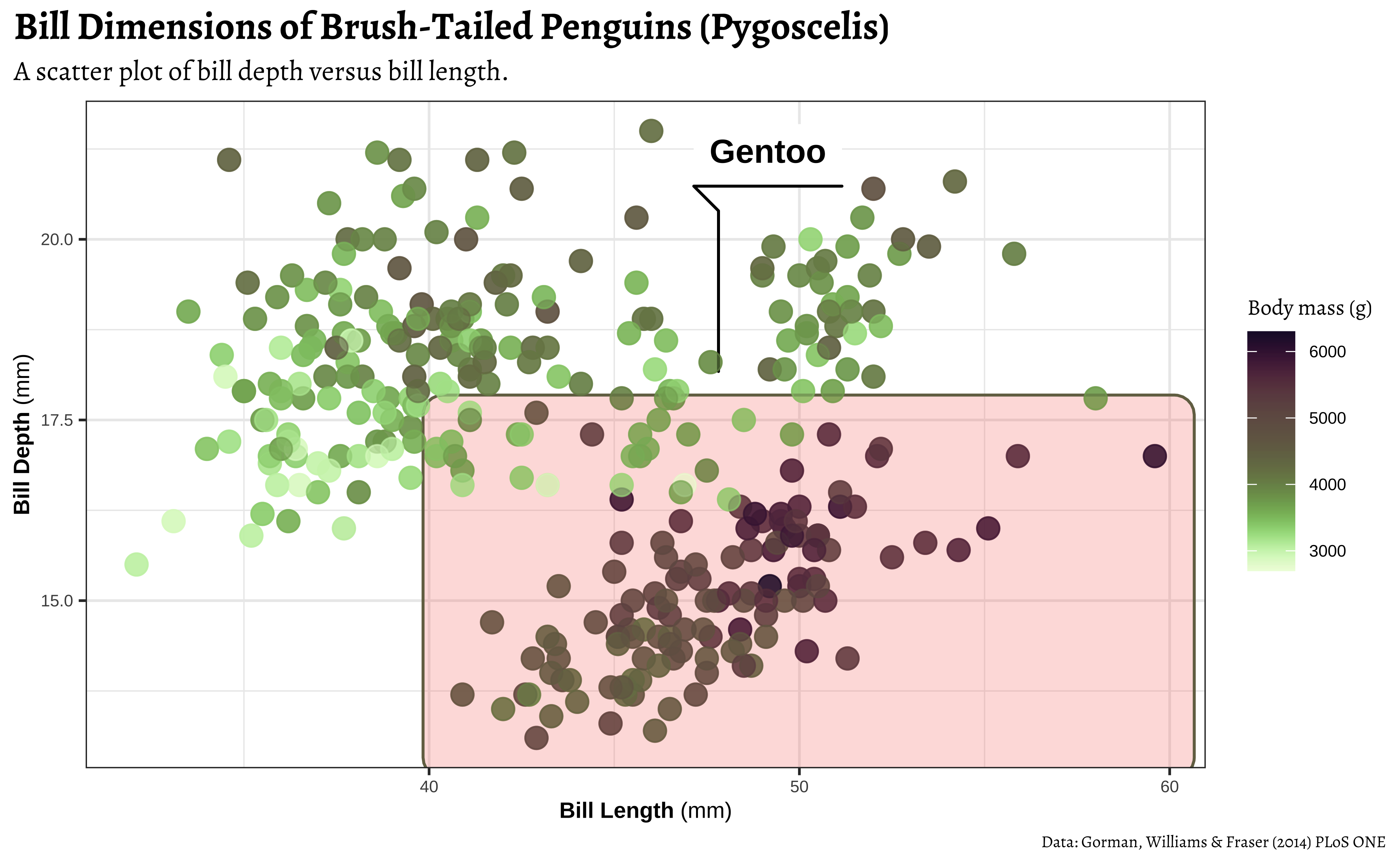
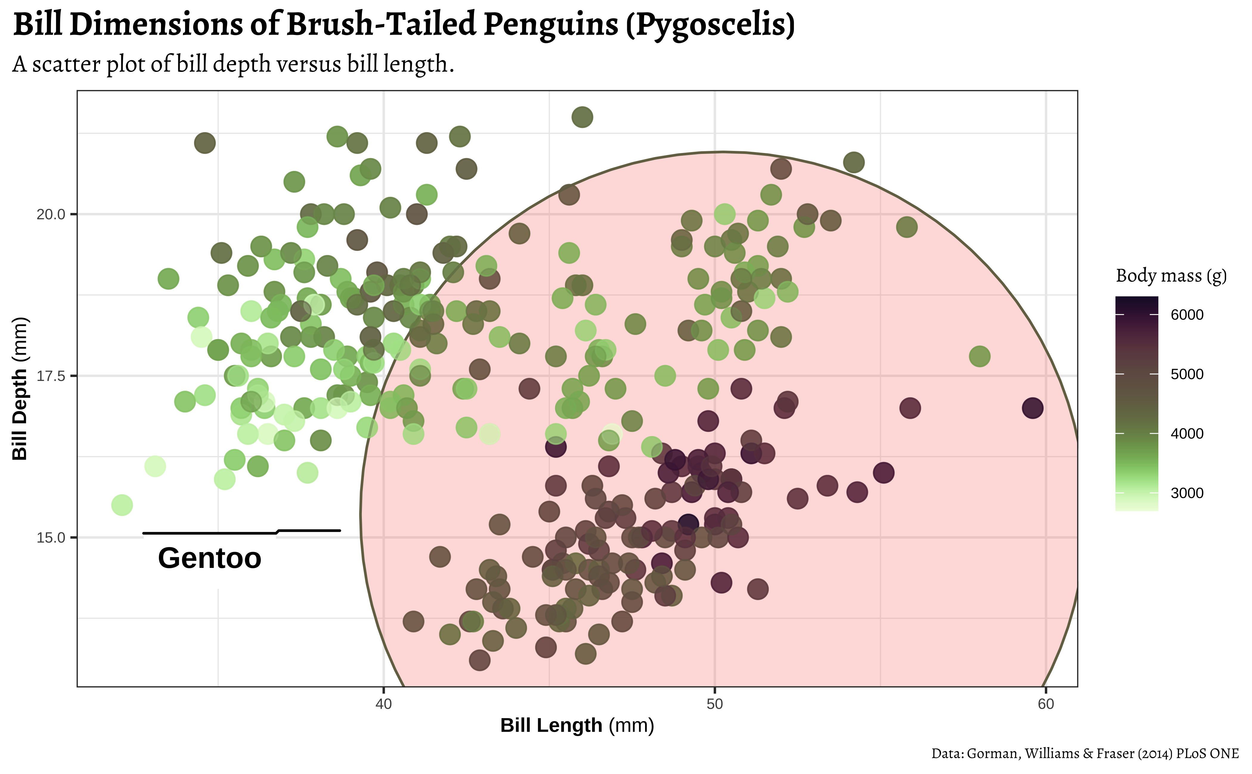
Annotations help to draw attention to specific parts or the graph, specific areas of interest that are useful in telling the story .
We have already seen the annotate() command from ggplot2 first ( and the new gf_annotate() from ggformula). Here we will look at some of the intriguing features from the ggdiagram package. We will also explore the ggforce package, and see if we can make our diagrams interactive with plotly.
1.1 Fonts and Themes
Show the Code
## Clean the slate
systemfonts::clear_local_fonts()
systemfonts::clear_registry()
##
showtext_opts(dpi = 96) # set DPI for showtext
sysfonts::font_add(
  family = "Alegreya",
  regular = "../../../../../../fonts/Alegreya-Regular.ttf",
  bold = "../../../../../../fonts/Alegreya-Bold.ttf",
  italic = "../../../../../../fonts/Alegreya-Italic.ttf",
  bolditalic = "../../../../../../fonts/Alegreya-BoldItalic.ttf"
)

sysfonts::font_add(
  family = "Anton",
  regular = "../../../../../../fonts/Anton-Regular.ttf"
) # Only one style is available

sysfonts::font_add(
  family = "RobotoCondensed",
  regular = "../../../../../../fonts/RobotoCondensed-Regular.ttf",
  bold = "../../../../../../fonts/RobotoCondensed-Bold.ttf",
  italic = "../../../../../../fonts/RobotoCondensed-Italic.ttf",
  bolditalic = "../../../../../../fonts/RobotoCondensed-BoldItalic.ttf"
)

sysfonts::font_add(
  family = "IbarraNova",
  regular = "../../../../../../fonts/IbarraRealNova-Regular.ttf",
  bold = "../../../../../../fonts/IbarraRealNova-Bold.ttf",
  italic = "../../../../../../fonts/IbarraRealNova-Italic.ttf",
  bolditalic = "../../../../../../fonts/IbarraRealNova-BoldItalic.ttf"
)

sysfonts::font_add(
  family = "Tangerine",
  regular = "../../../../../../fonts/Tangerine-Regular.ttf",
  bold = "../../../../../../fonts/Tangerine-Bold.ttf"
) # only these two are available

sysfonts::font_add(
  family = "Schoolbell",
  regular = "../../../../../../fonts/Schoolbell-Regular.ttf"
) # Only regular is available

showtext_auto() # set these fonts as default for the session
# sysfonts::font_families() # check which fonts are available in the session
2 Set the Theme
Show the Code
theme_custom <- function() {
  theme_bw(base_size = 10) +

    theme_sub_axis(
      title = element_text(
        family = "Roboto Condensed",
        size = 8
      ),
      text = element_text(
        family = "Roboto Condensed",
        size = 6
      )
    ) +

    theme_sub_legend(
      text = element_text(
        family = "Roboto Condensed",
        size = 6
      ),
      title = element_text(
        family = "Alegreya",
        size = 8
      )
    ) +

    theme_sub_plot(
      title = element_text(
        family = "Alegreya",
        size = 14, face = "bold"
      ),
      title.position = "plot",
      subtitle = element_text(
        family = "Alegreya",
        size = 10
      ),
      caption = element_text(
        family = "Alegreya",
        size = 6
      ),
      caption.position = "plot"
    )
}

## Use available fonts in ggplot text geoms too!
ggplot2::update_geom_defaults(geom = "text", new = list(
  family = "Roboto Condensed",
  face = "plain",
  size = 3.5,
  color = "#2b2b2b"
))
ggplot2::update_geom_defaults(geom = "label", new = list(
  family = "Roboto Condensed",
  face = "plain",
  size = 3.5,
  color = "#2b2b2b"
))

ggplot2::update_geom_defaults(geom = "marquee", new = list(
  family = "Roboto Condensed",
  face = "plain",
  size = 3.5,
  color = "#2b2b2b"
))
ggplot2::update_geom_defaults(geom = "text_repel", new = list(
  family = "Roboto Condensed",
  face = "plain",
  size = 3.5,
  color = "#2b2b2b"
))
ggplot2::update_geom_defaults(geom = "label_repel", new = list(
  family = "Roboto Condensed",
  face = "plain",
  size = 3.5,
  color = "#2b2b2b"
))

## Set the theme
ggplot2::theme_set(new = theme_custom())

## tinytable options
options("tinytable_tt_digits" = 2)
options("tinytable_format_num_fmt" = "significant_cell")
options(tinytable_html_mathjax = TRUE)


## Set defaults for flextable
flextable::set_flextable_defaults(font.family = "Roboto Condensed")
3
ggdiagram is a relatively new package in R that exploits some of the more recent developments in the R core. It uses for example, a new Object Oriented System in R called S7 that allows commands to be “cascaded” in a way similar to Python and Javascript. Its best feature is that it allows precise control of shapes, their locations and connections, and returns a ggplot chart at the end, allowing us to use all the ggplot skills and bells and whistles, should we need them.
The webpage for ggdiagram is at https://wjschne.github.io/ggdiagram/
4 Method
ggdiagram allows to create diverse shapes, and then connect them together as we need.
The method we will use is as follows: Define -> Place -> Connect:
- pre-create the shapes we need and save them as variables
- place the shapes in relation to each other using
ggdiagram::place(); - invoke
ggdiagram()and thenggdiagram::connect()the shapes we have created in the and manner that we need.
4.1 Basic Shapes in {ggdiagram}

s1 <- ob_rectangle()
ggdiagram() + s1
r1 <- ob_reuleaux(fill = "white")
ggdiagram() + r1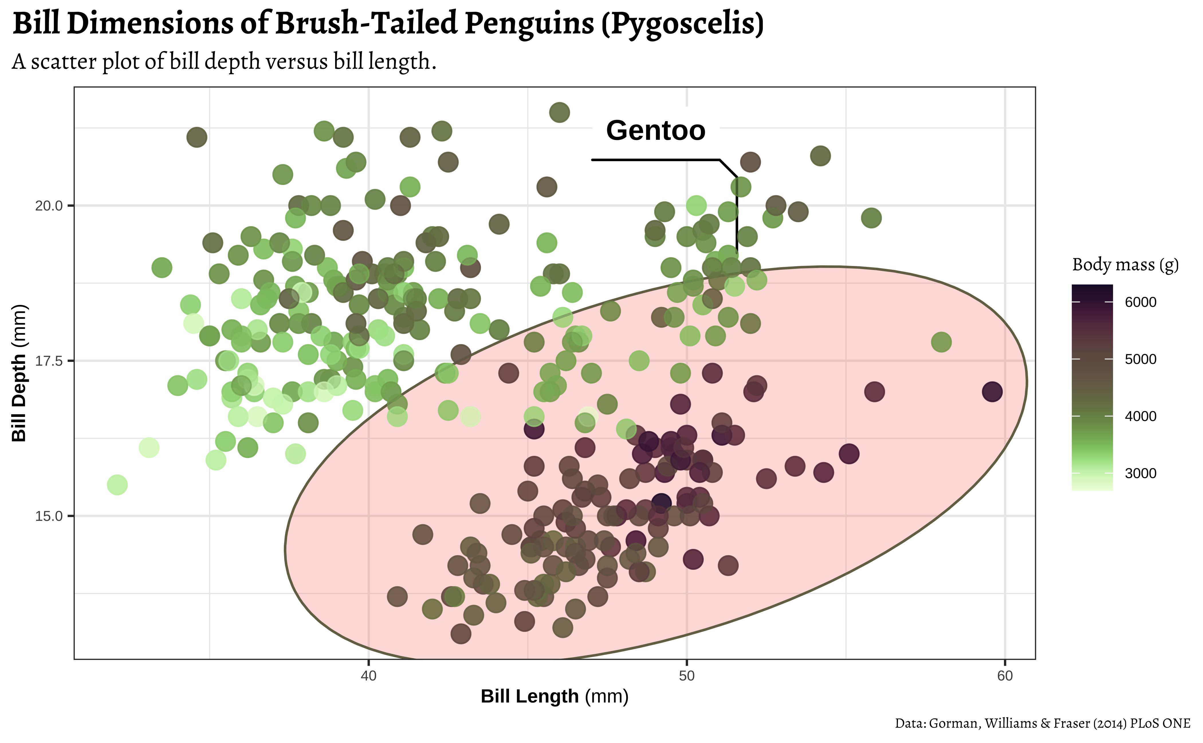
4.2 Placement
4.3 Connecting Shapes
# 1) Define shapes
start <- ob_circle(radius = 0.5)
decision <- ob_rectangle(width = 2.0, height = 1.0)
end <- ob_circle(radius = 0.5)

# 2) Place shapes
decision <- decision %>% place(from = start, where = "right", sep = 1.5)
end <- end %>% place(from = decision, where = "right", sep = 1.5)

# 3) Draw diagram
ggdiagram() +
  start +
  decision +
  end +
  connect(start, decision) +
  connect(decision, end) +
  coord_fixed() +
  theme_void()