1 Setting up R Packages
Plot Fonts and Theme
Show the Code
library(systemfonts)
library(showtext)
## Clean the slate
systemfonts::clear_local_fonts()
systemfonts::clear_registry()
##
showtext_opts(dpi = 96) # set DPI for showtext
sysfonts::font_add(
  family = "Alegreya",
  regular = "../../../../../../fonts/Alegreya-Regular.ttf",
  bold = "../../../../../../fonts/Alegreya-Bold.ttf",
  italic = "../../../../../../fonts/Alegreya-Italic.ttf",
  bolditalic = "../../../../../../fonts/Alegreya-BoldItalic.ttf"
)

sysfonts::font_add(
  family = "Roboto Condensed",
  regular = "../../../../../../fonts/RobotoCondensed-Regular.ttf",
  bold = "../../../../../../fonts/RobotoCondensed-Bold.ttf",
  italic = "../../../../../../fonts/RobotoCondensed-Italic.ttf",
  bolditalic = "../../../../../../fonts/RobotoCondensed-BoldItalic.ttf"
)
showtext_auto(enable = TRUE) # enable showtext
##
theme_custom <- function() {
  font <- "Alegreya" # assign font family up front
  "%+replace%" <- ggplot2::"%+replace%" # nolint

  theme_classic(base_size = 14, base_family = font) %+replace% # replace elements we want to change

    theme(
      text = element_text(family = font), # set base font family

      # text elements
      plot.title = element_text( # title
        family = font, # set font family
        size = 24, # set font size
        face = "bold", # bold typeface
        hjust = 0, # left align
        margin = margin(t = 5, r = 0, b = 5, l = 0)
      ), # margin
      plot.title.position = "plot",
      plot.subtitle = element_text( # subtitle
        family = font, # font family
        size = 14, # font size
        hjust = 0, # left align
        margin = margin(t = 5, r = 0, b = 10, l = 0)
      ), # margin

      plot.caption = element_text( # caption
        family = font, # font family
        size = 9, # font size
        hjust = 1
      ), # right align

      plot.caption.position = "plot", # right align

      axis.title = element_text( # axis titles
        family = "Roboto Condensed", # font family
        size = 12
      ), # font size

      axis.text = element_text( # axis text
        family = "Roboto Condensed", # font family
        size = 9
      ), # font size

      axis.text.x = element_text( # margin for axis text
        margin = margin(5, b = 10)
      )

      # since the legend often requires manual tweaking
      # based on plot content, don't define it here
    )
}

## Use available fonts in ggplot text geoms too!
ggplot2::update_geom_defaults(geom = "text", new = list(
  family = "Roboto Condensed",
  face = "plain",
  size = 3.5,
  color = "#2b2b2b"
))
ggplot2::update_geom_defaults(geom = "label", new = list(
  family = "Roboto Condensed",
  face = "plain",
  size = 3.5,
  color = "#2b2b2b"
))

## Set the theme
ggplot2::theme_set(new = theme_custom())
2 Introduction
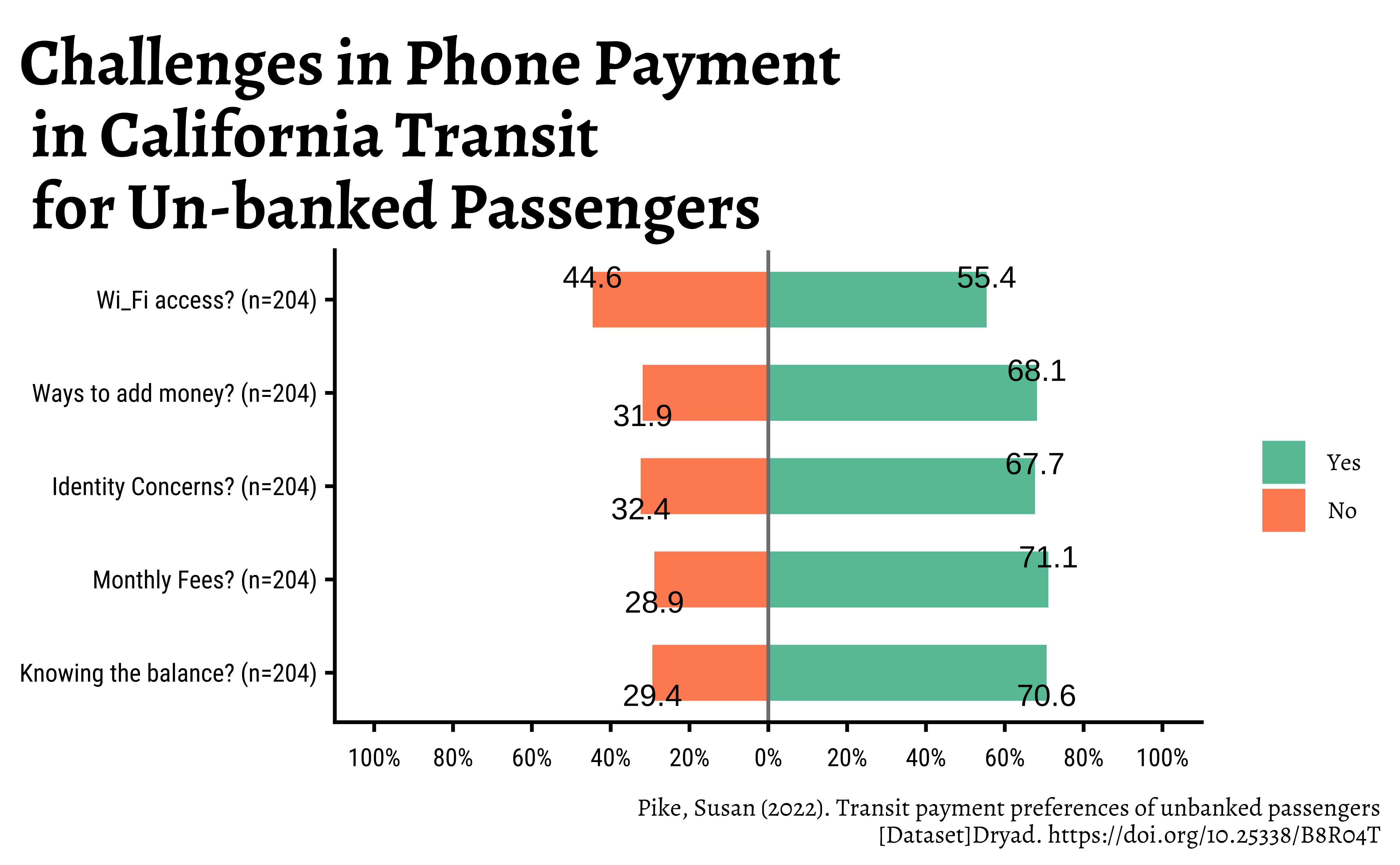
This dataset is the result of a research study on payment options for people using public transit in California.
The dataset is available on Dataset Dryad:
Pike, Susan (2022). Transit payment preferences of unbanked passengers. Dataset Dryad. https://doi.org/10.25338/B8R04T
And a brief 2-pager on the research methodology is here.
Yes, peasants, you should read such stuff from other very different domains!
3 Read the Data
4 Data Dictionary
NoteQuantitative Variables
Write in.
NoteQualitative Variables
Write in.
NoteObservations
Write in.
5 Data Munging
Munged Data
6 Summarize and Prepare the Data
Let’s label the data variables…
tibble [204 × 5] (S3: tbl_df/tbl/data.frame)
 $ phone.wifi    : num [1:204] 1 1 2 1 1 2 1 1 1 2 ...
  ..- attr(*, "label")= Named chr "Wi_Fi access?"
  .. ..- attr(*, "names")= chr "phone.wifi"
  ..- attr(*, "labels")= Named num [1:2] 1 2
  .. ..- attr(*, "names")= chr [1:2] "No" "Yes"
 $ phone.money   : num [1:204] 1 1 1 1 1 1 1 1 1 2 ...
  ..- attr(*, "label")= Named chr "Ways to add money?"
  .. ..- attr(*, "names")= chr "phone.money"
  ..- attr(*, "labels")= Named num [1:2] 1 2
  .. ..- attr(*, "names")= chr [1:2] "No" "Yes"
 $ phone.identity: num [1:204] 1 1 2 2 1 1 2 1 1 2 ...
  ..- attr(*, "label")= Named chr "Identity Concerns?"
  .. ..- attr(*, "names")= chr "phone.identity"
  ..- attr(*, "labels")= Named num [1:2] 1 2
  .. ..- attr(*, "names")= chr [1:2] "No" "Yes"
 $ phone.fees    : num [1:204] 1 2 1 1 1 1 1 1 1 1 ...
  ..- attr(*, "label")= Named chr "Monthly Fees?"
  .. ..- attr(*, "names")= chr "phone.fees"
  ..- attr(*, "labels")= Named num [1:2] 1 2
  .. ..- attr(*, "names")= chr [1:2] "No" "Yes"
 $ phone.balance : num [1:204] 1 2 1 1 1 1 1 2 1 2 ...
  ..- attr(*, "label")= Named chr "Knowing the balance?"
  .. ..- attr(*, "names")= chr "phone.balance"
  ..- attr(*, "labels")= Named num [1:2] 1 2
  .. ..- attr(*, "names")= chr [1:2] "No" "Yes"
7 Plot the Data
8 Task and Discussion
Complete the Data Dictionary. Select and Transform the variables as shown. Create the graph shown below and discuss the following questions:
- Identify the type of charts
- Identify the variables used for various geometrical aspects (x, y, fill…). Name the variables appropriately.
- What activity might have been carried out to obtain the data graphed here? Provide some details.
- What would be your recommendation to the Transport Company?
- To the Phone Companies?