The Mad Hatter’s Guide to Data Viz and Stats in R
  1. ANOVA - Tyre Brands and Mileage
  • Data Viz and Stats
    • Tools
      • Introduction to R and RStudio
    • Studio Flow and Data Kits
      • 12-Day Studio Index
      • Healthcare Data Kits
    • Visualization
      • Data
      • Inspect Data
      • Graphs
      • Summaries
      • Counts
      • Quantities
      • Groups
      • Distributions
      • Groups and Distributions
      • Change
      • Proportions
      • Hierarchy
      • Evolution and Flow
      • Ratings and Rankings
      • Surveys
      • Time
      • Space
        • Introduction to Maps
        • What is Vector Data?
        • The Grammar of Maps
        • Interactive Maps with leaflet
      • Networks
      • Miscellaneous Graphing Tools, and References
    • Inference
      • Basics
      • 🎲 Samples
      • Randomization
      • One Mean
      • Two Independent Means
      • Two Paired Means
      • Multiple Means (ANOVA)
      • Correlation
      • One Proportion
      • Two Proportions
    • Modelling
      • Linear Regression
      • Logistic Regression
      • 🕔 Time Series
    • Workflow
      • Facing the Abyss
      • I Publish, therefore I Am
      • Data Carpentry
    • Arts
      • Colours
      • Fonts for Charts
      • Font Effects in Charts
      • Branding and Typography
      • Annotations
      • More Annotations
      • Highlighting
      • Scales
    • AI Tools
      • Using gander and ellmer
      • Using Github Copilot and other AI tools to generate R code
      • Using LLMs to Explain Stat models
    • Case Studies
      • Demo:Product Packaging and Elderly People
      • Ikea Furniture
      • Movie Profits
      • Gender at the Work Place
      • Heptathlon
      • School Scores
      • Children's Games
      • Valentine’s Day Spending
      • Women Live Longer?
      • Hearing Loss in Children
      • California Transit Payments
      • Seaweed Nutrients
      • Coffee Flavours
      • Legionnaire’s Disease in the USA
      • Antarctic Sea ice
      • William Farr's Observations on Cholera in London
    • Projects
      • No Free Hunch

On this page

  • 1 Setting up R Packages
  • 2 Introduction
  • 3 Data
  • 4 Download the Modified data
  • 5 Data Dictionary
  • 6 Plot the Data
  • 7 Task and Discussion: ANOVA
    • 7.1 Model + Table
    • 7.2 Post-hoc Analysis and Plots
    • 7.3 Conclusion

ANOVA - Tyre Brands and Mileage

1 Setting up R Packages

library(tidyverse)
library(mosaic)
library(skimr)
library(ggformula)
library(ggprism) # Interesting Categorical Axes
library(ggridges)
library(supernova)
# devtools::install_github('cttobin/ggthemr')
library(ggthemr)
Error in `library()`:
! there is no package called 'ggthemr'
library(ggsci)
Error in `library()`:
! there is no package called 'ggthemr'

Plot Fonts and Theme

Show the Code
source(here::here("R", "theme-hatter.R")) # fonts, geom/table defaults, themes
theme_custom <- theme_hatter_alegreya # same design this page used to define locally
ggplot2::theme_set(new = theme_custom())

2 Introduction

This is a dataset pertaining to tyres from different companies and their lifetime mileages.

3 Data

4 Download the Modified data

5 Data Dictionary

NoteQuantitative Variables

Write in.

NoteQualitative Variables

Write in.

NoteObservations

Write in.

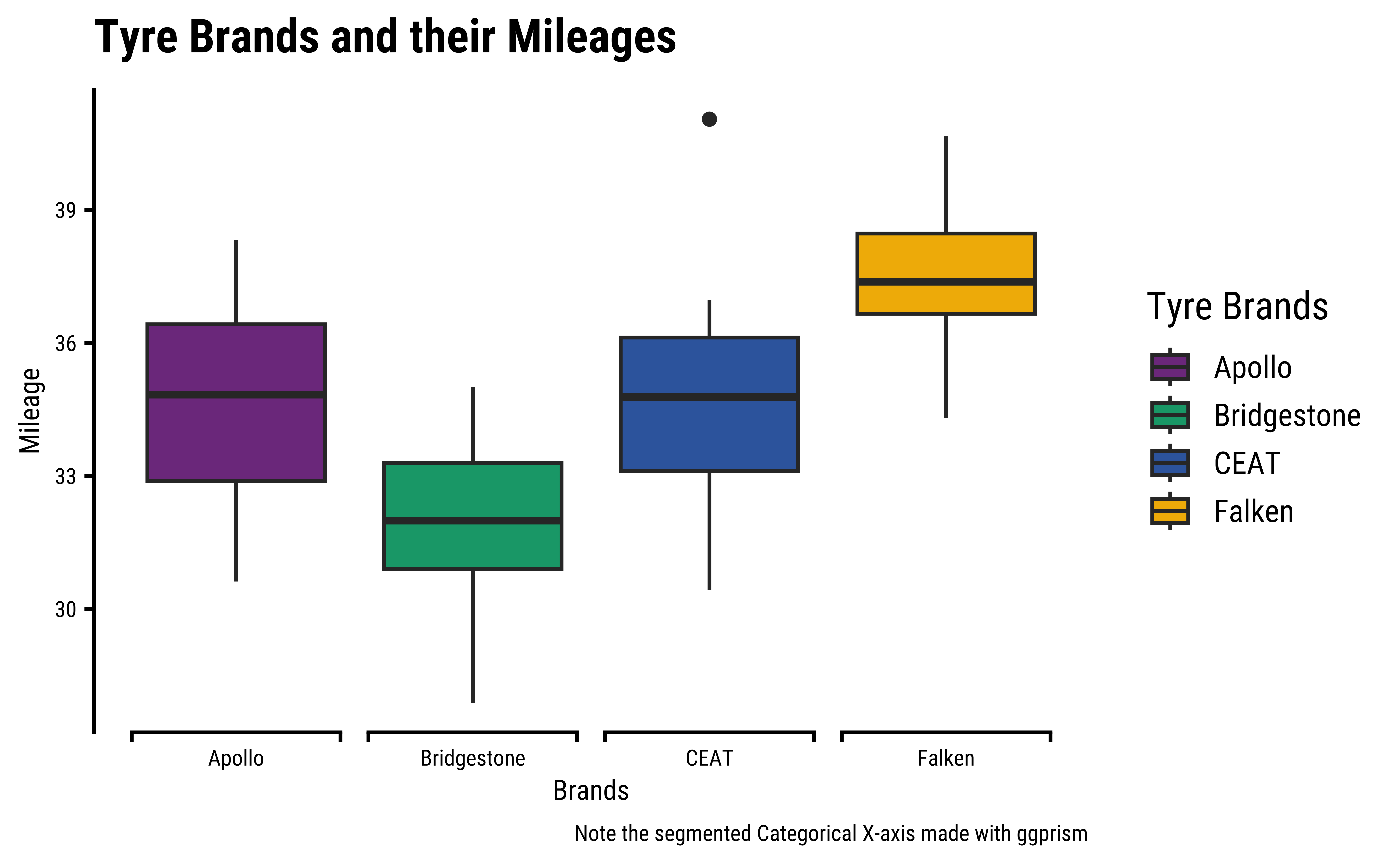
6 Plot the Data
7 Task and Discussion: ANOVA

  1. Complete the pre-analysis steps for ANOVA

Write in.

7.1 Model + Table

  1. Create the ANOVA model
  2. Create the ANOVA table using the supernova package
Call:
   aov(formula = Mileage ~ Brands, data = tyre)

Terms:
                  Brands Residuals
Sum of Squares  256.2908  266.6495
Deg. of Freedom        3        56

Residual standard error: 2.182108
Estimated effects may be unbalanced
 Analysis of Variance Table (Type III SS)
 Model: Mileage ~ Brands

                              SS df     MS      F   PRE     p
 ----- --------------- | ------- -- ------ ------ ----- -----
 Model (error reduced) | 256.291  3 85.430 17.942 .4901 .0000
 Error (from model)    | 266.649 56  4.762                   
 ----- --------------- | ------- -- ------ ------ ----- -----
 Total (empty model)   | 522.940 59  8.863                   

7.2 Post-hoc Analysis and Plots

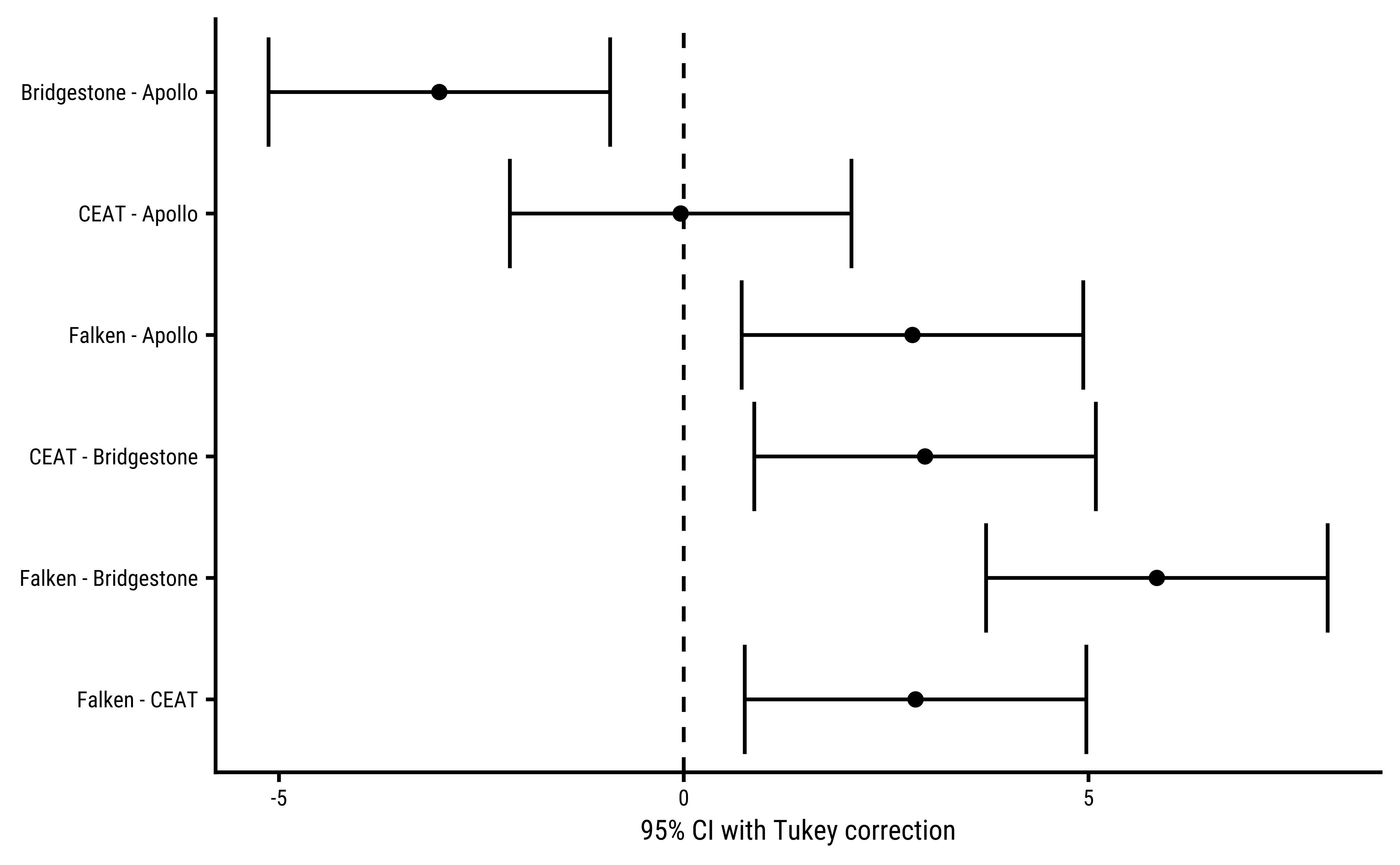
  1. Compute the post-hoc differences in means and plot the pair-wise difference plots

  group_1     group_2       diff pooled_se      q    df  lower  upper  p_adj
  <chr>       <chr>        <dbl>     <dbl>  <dbl> <int>  <dbl>  <dbl>  <dbl>
1 Bridgestone Apollo      -3.019     0.563 -5.358    56 -5.129 -0.909  .0021
2 CEAT        Apollo      -0.038     0.563 -0.067    56 -2.148  2.072 1.0000
3 Falken      Apollo       2.826     0.563  5.015    56  0.716  4.935  .0043
4 CEAT        Bridgestone  2.981     0.563  5.291    56  0.871  5.091  .0024
5 Falken      Bridgestone  5.845     0.563 10.373    56  3.735  7.954  .0000
6 Falken      CEAT         2.863     0.563  5.082    56  0.754  4.973  .0037
7.3 Conclusion

  1. State a conclusion about the effect of Brands on Mileage.

Write in.

Back to top

License: CC BY-SA 2.0

Website made with ❤️ and Quarto, by Arvind V.

Hosted by Netlify .