1 Setting up R Packages
Plot Fonts and Theme
Show the Code
library(systemfonts)
library(showtext)
## Clean the slate
systemfonts::clear_local_fonts()
systemfonts::clear_registry()
##
showtext_opts(dpi = 96) # set DPI for showtext
sysfonts::font_add(
  family = "Alegreya",
  regular = "../../../../../../fonts/Alegreya-Regular.ttf",
  bold = "../../../../../../fonts/Alegreya-Bold.ttf",
  italic = "../../../../../../fonts/Alegreya-Italic.ttf",
  bolditalic = "../../../../../../fonts/Alegreya-BoldItalic.ttf"
)

sysfonts::font_add(
  family = "Roboto Condensed",
  regular = "../../../../../../fonts/RobotoCondensed-Regular.ttf",
  bold = "../../../../../../fonts/RobotoCondensed-Bold.ttf",
  italic = "../../../../../../fonts/RobotoCondensed-Italic.ttf",
  bolditalic = "../../../../../../fonts/RobotoCondensed-BoldItalic.ttf"
)
showtext_auto(enable = TRUE) # enable showtext
##
theme_custom <- function() {
  font <- "Alegreya" # assign font family up front
  "%+replace%" <- ggplot2::"%+replace%" # nolint

  theme_classic(base_size = 14, base_family = font) %+replace% # replace elements we want to change

    theme(
      text = element_text(family = font), # set base font family

      # text elements
      plot.title = element_text( # title
        family = font, # set font family
        size = 24, # set font size
        face = "bold", # bold typeface
        hjust = 0, # left align
        margin = margin(t = 5, r = 0, b = 5, l = 0)
      ), # margin
      plot.title.position = "plot",
      plot.subtitle = element_text( # subtitle
        family = font, # font family
        size = 14, # font size
        hjust = 0, # left align
        margin = margin(t = 5, r = 0, b = 10, l = 0)
      ), # margin

      plot.caption = element_text( # caption
        family = font, # font family
        size = 9, # font size
        hjust = 1
      ), # right align

      plot.caption.position = "plot", # right align

      axis.title = element_text( # axis titles
        family = "Roboto Condensed", # font family
        size = 12
      ), # font size

      axis.text = element_text( # axis text
        family = "Roboto Condensed", # font family
        size = 9
      ), # font size

      axis.text.x = element_text( # margin for axis text
        margin = margin(5, b = 10)
      )

      # since the legend often requires manual tweaking
      # based on plot content, don't define it here
    )
}

## Use available fonts in ggplot text geoms too!
ggplot2::update_geom_defaults(geom = "text", new = list(
  family = "Roboto Condensed",
  face = "plain",
  size = 3.5,
  color = "#2b2b2b"
))

## Set the theme
ggplot2::theme_set(new = theme_custom())
2 Introduction
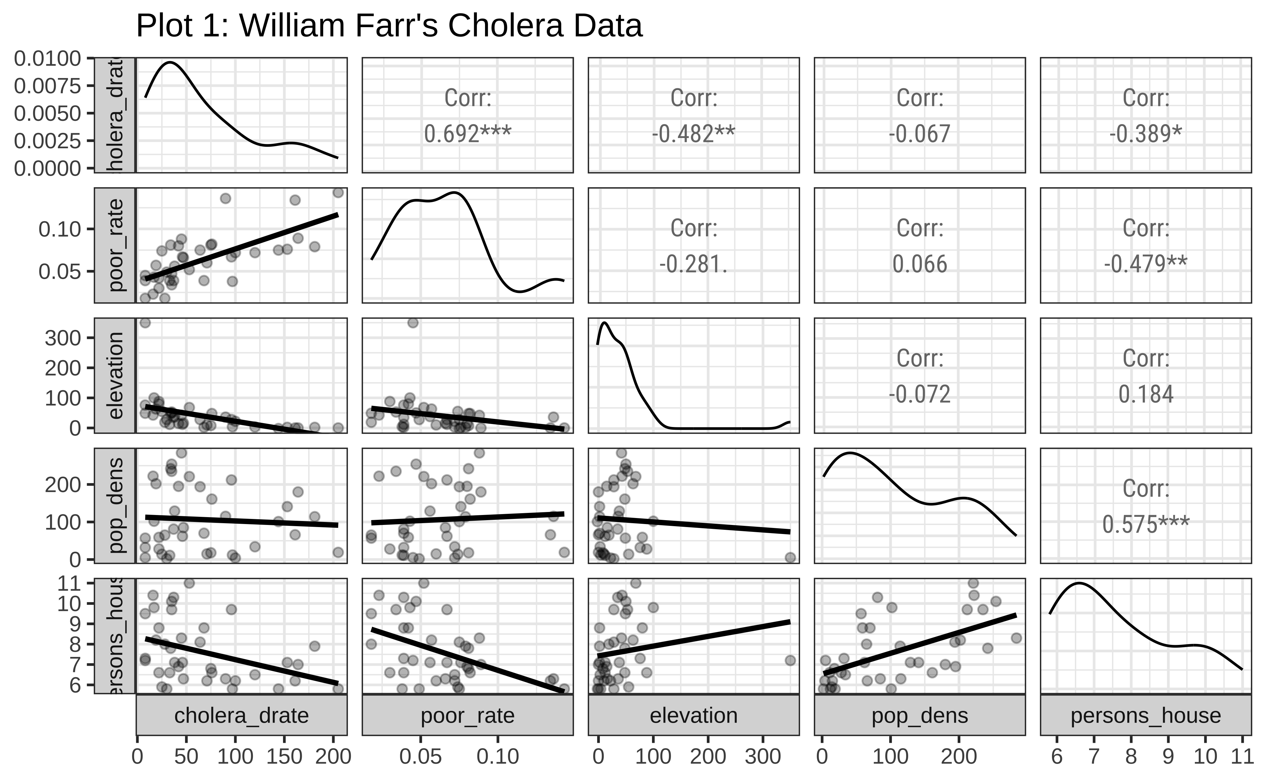
John Snow’s contention that cholera was principally spread by water was not accepted in the 1850s by the medical elite. The consequence of rejection was that hundreds in the UK continued to die. William Farr, who founded the science of epidemiology, tried to examine if there were other causes that led to cholera. He had concluded that the available data not only supported miasma (spread via atmospheric vapours) but also indicated that there was an underlying ‘natural law’ linking infection with cholera inversely to elevation above high water. The data is available on Vincent Arel-Bundock’s website, and is part of the HistData package from Michael Friendly, UC Davis.
3 Read the Data
Cholera <- read_csv("https://vincentarelbundock.github.io/Rdatasets/csv/HistData/Cholera.csv")
Cholera
4 Data Dictionary
NoteQuantitative Variables
Write in.
NoteQualitative Variables
Write in.
NoteObservations
Write in.
5 Research Question
Note
Write in! Look at the charts below!
6 Analyse/Transform the Data
```{r}
#| label: data-preprocessing
#
# Write in your code here
# to prepare this data as shown below
# to generate the plot that follows
```
7 Plot the Data
8 Tasks and Discussion
- Complete the Data Dictionary.
- Select and Transform the variables as needed.
- Look at Plot 1. Would you agree based on this chart that William Farr was right in believing that elevation was a good predictor for cholera deaths? Justify.
- What is the nature of the relationship between Cholera Deaths and Elevation?
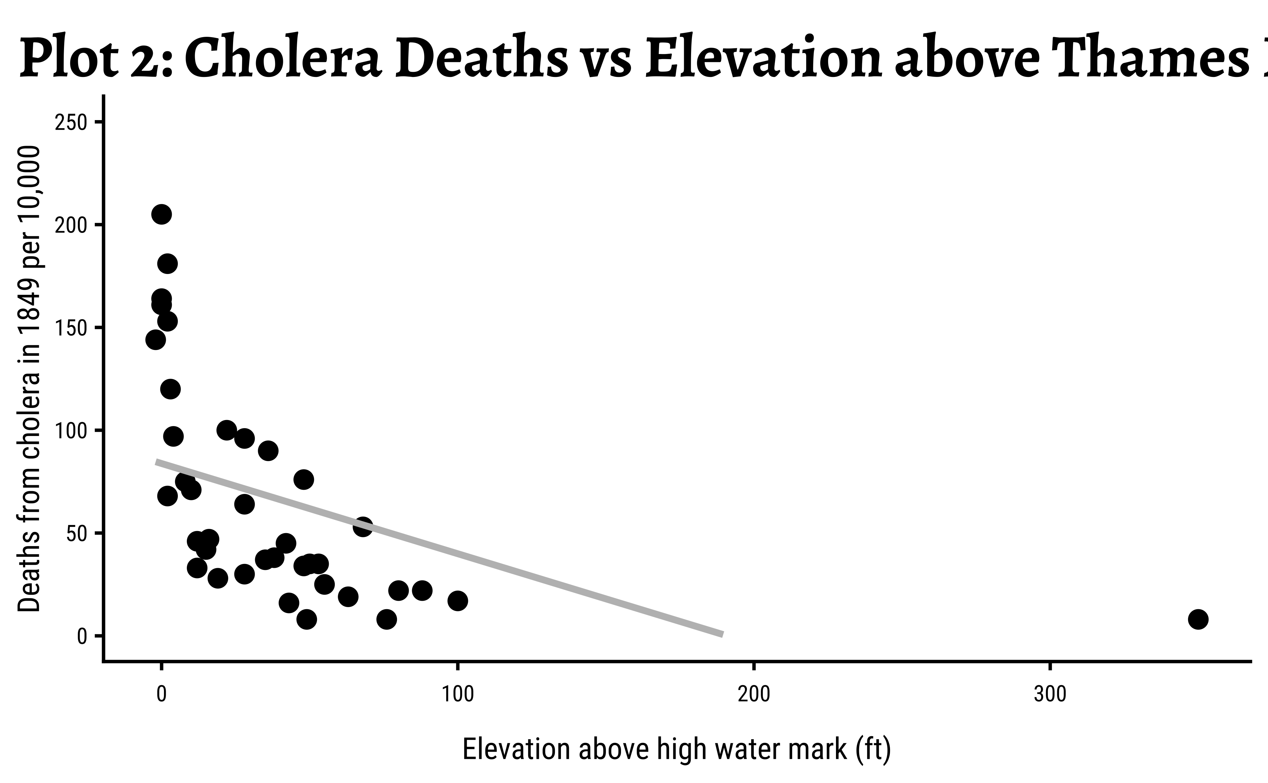
- Look at Plot 2. What kind of plot is it? What is the relationship here between Elevation and Cholera Death Rate?
- Based on this graph, would you agree that Elevation is a predictor for Cholera Deaths? Justify.
- Is the relationship you found between Cholera Deaths and Elevation also found in Plot 1? Justify.
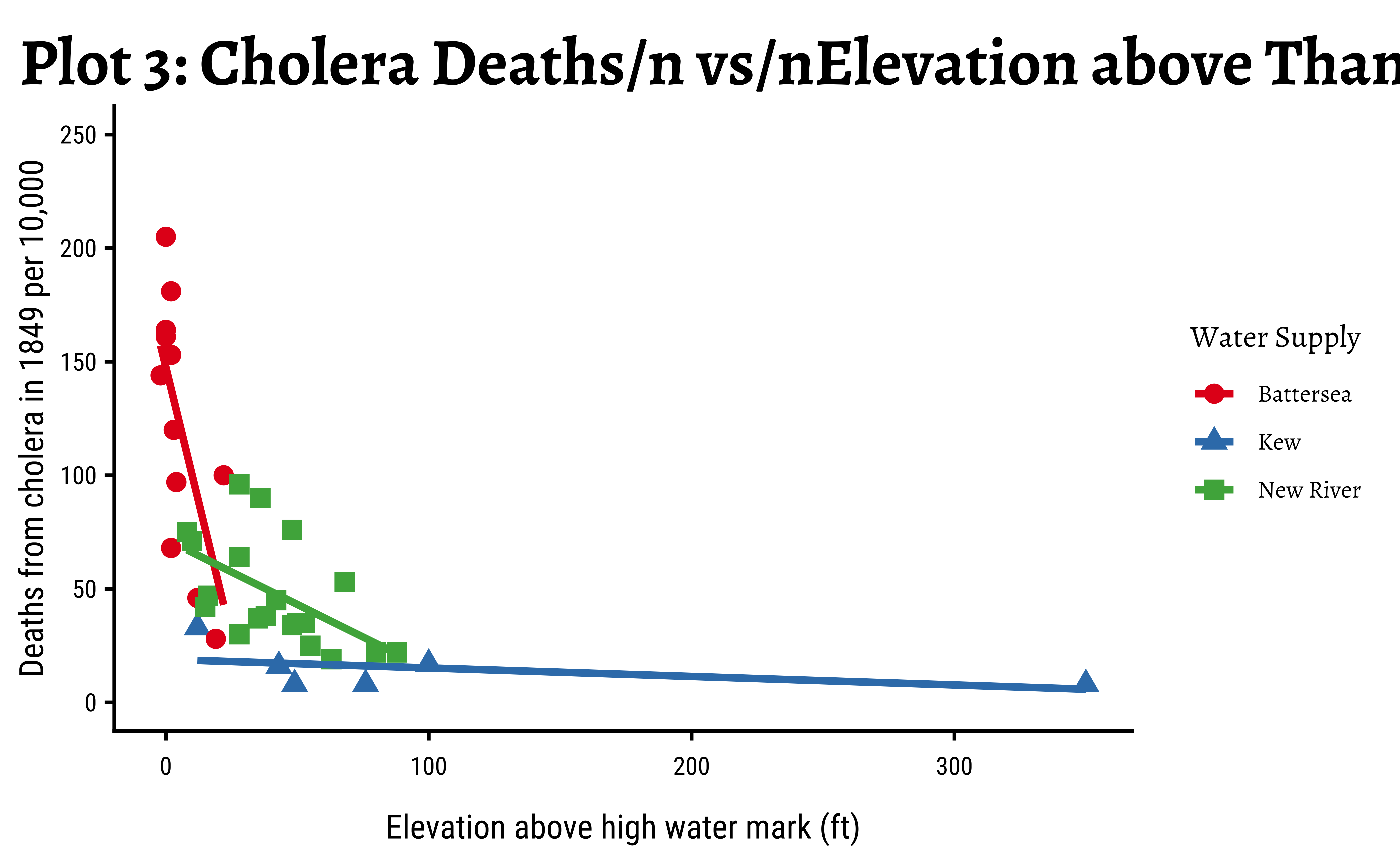
- Look at Plot 3. Would you guess that there could be another predictor for Cholera Deaths? What could that Predictor be? Justify.