The Mad Hatter’s Guide to Data Viz and Stats in R
  1. Correlation and Regression Explorations
  • Data Viz and Stats
    • Tools
      • Introduction to R and RStudio
    • Studio Flow and Data Kits
      • 12-Day Studio Index
      • Healthcare Data Kits
    • Visualization
      • Data
      • Inspect Data
      • Graphs
      • Summaries
      • Counts
      • Quantities
      • Groups
      • Distributions
      • Groups and Distributions
      • Change
      • Proportions
      • Hierarchy
      • Evolution and Flow
      • Ratings and Rankings
      • Surveys
      • Time
      • Space
        • Introduction to Maps
        • What is Vector Data?
        • The Grammar of Maps
        • Interactive Maps with leaflet
      • Networks
      • Miscellaneous Graphing Tools, and References
    • Inference
      • Basics
      • 🎲 Samples
      • Randomization
      • One Mean
      • Two Independent Means
      • Two Paired Means
      • Multiple Means (ANOVA)
      • Correlation
      • One Proportion
      • Two Proportions
    • Modelling
      • Linear Regression
      • Logistic Regression
      • 🕔 Time Series
    • Workflow
      • Facing the Abyss
      • I Publish, therefore I Am
      • Data Carpentry
    • Arts
      • Colours
      • Fonts for Charts
      • Font Effects in Charts
      • Branding and Typography
      • Annotations
      • More Annotations
      • Highlighting
      • Scales
    • AI Tools
      • Using gander and ellmer
      • Using Github Copilot and other AI tools to generate R code
      • Using LLMs to Explain Stat models
    • Case Studies
      • Demo:Product Packaging and Elderly People
      • Ikea Furniture
      • Movie Profits
      • Gender at the Work Place
      • Heptathlon
      • School Scores
      • Children's Games
      • Valentine’s Day Spending
      • Women Live Longer?
      • Hearing Loss in Children
      • California Transit Payments
      • Seaweed Nutrients
      • Coffee Flavours
      • Legionnaire’s Disease in the USA
      • Antarctic Sea ice
      • William Farr's Observations on Cholera in London
    • Projects
      • No Free Hunch

On this page

  • 1 Setting up R Packages
  • 2 Intro
  • 3 Explorations into Diagnostic Plots
    • 3.1 Normal Errors
    • 3.2 Uniform Errors
    • 3.3 Negative Binom Errors
    • 3.4 Gamma Errors

Correlation and Regression Explorations

Published

May 3, 2023

Modified

November 3, 2026

1 Setting up R Packages

library(tidyverse)
library(mosaic)
library(broom)
library(ggformula)

2 Intro

I will work through and “unify” at least two things:

  • Hadley Wickham’s chapter on modelling and his analysis of the linear model for the diamonds dataset
  • The diagnostic aspects of Linear Regression as detailed in Crawley’s book

3 Explorations into Diagnostic Plots

Let us create dependent y* variables with different sorts of errors:
x <- 0:300
en <- rnorm(301, mean = 0, sd = 5)
eu <- (runif(n = 301) - 0.5) * 20
eb <- rnbinom(n = 301, prob = 0.3, size = 2)
eg <- rgamma(n = 301, shape = 1, rate = 1 / x)
yn <- x + 10 + en
yu <- x + 10 + eu
yb <- x + 10 + eb
yg <- x + 10 + eg
data <- tibble(x, yn, yu, yb, yg)
data

3.1 Normal Errors

lm_norm_aug <- lm(yn ~ x, data = data) %>%
  augment()
lm_norm_aug %>% gf_point(.resid ~ .fitted)

lm_norm_aug %>%
  gf_qq(~.resid) %>%
  gf_qqline()

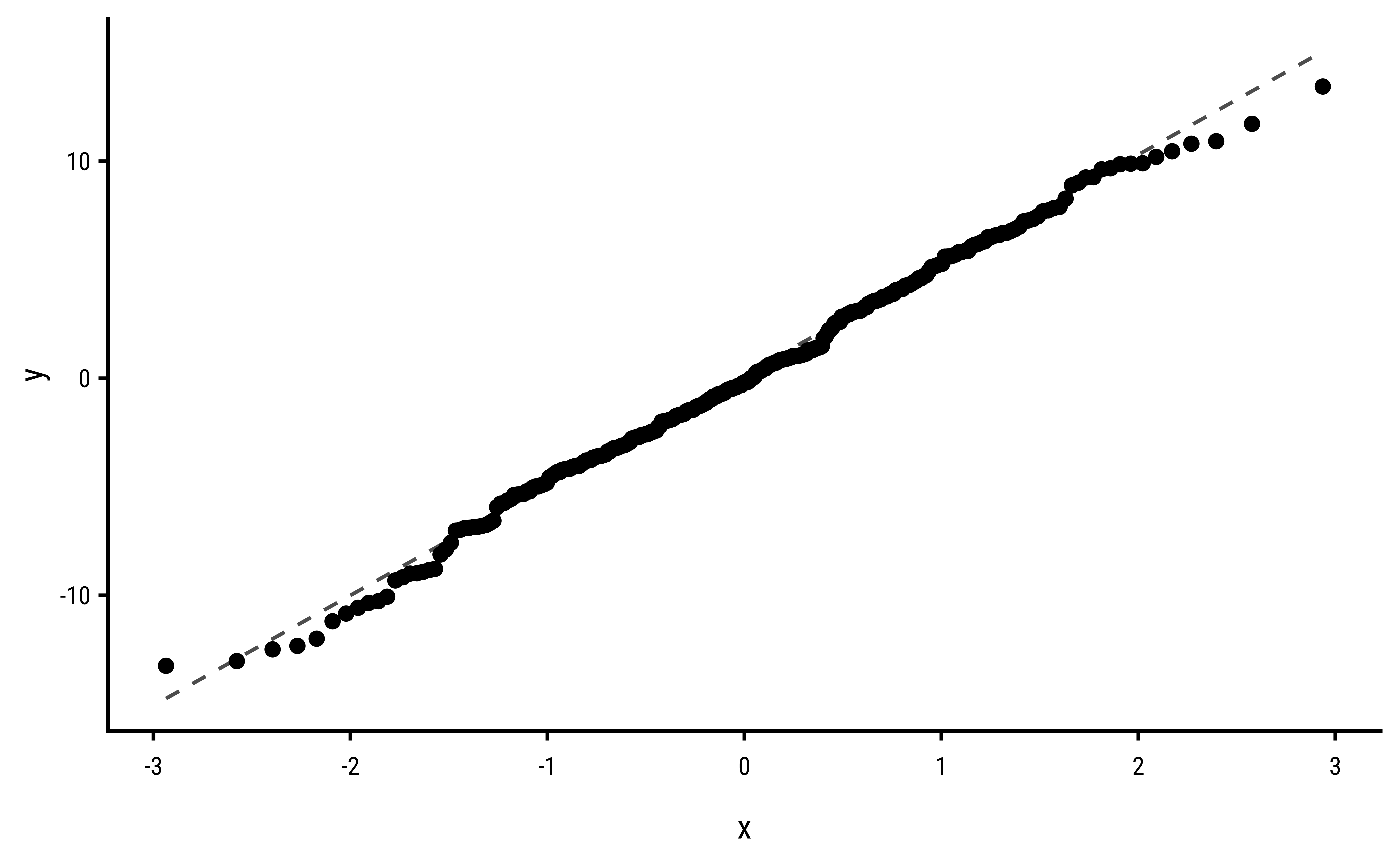
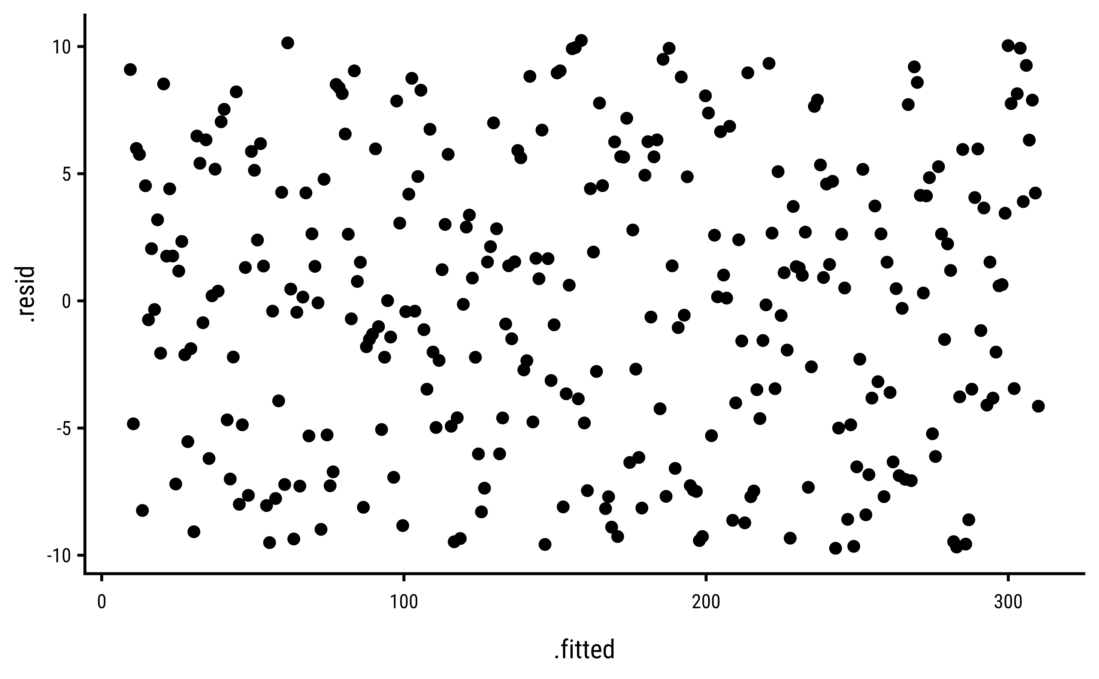
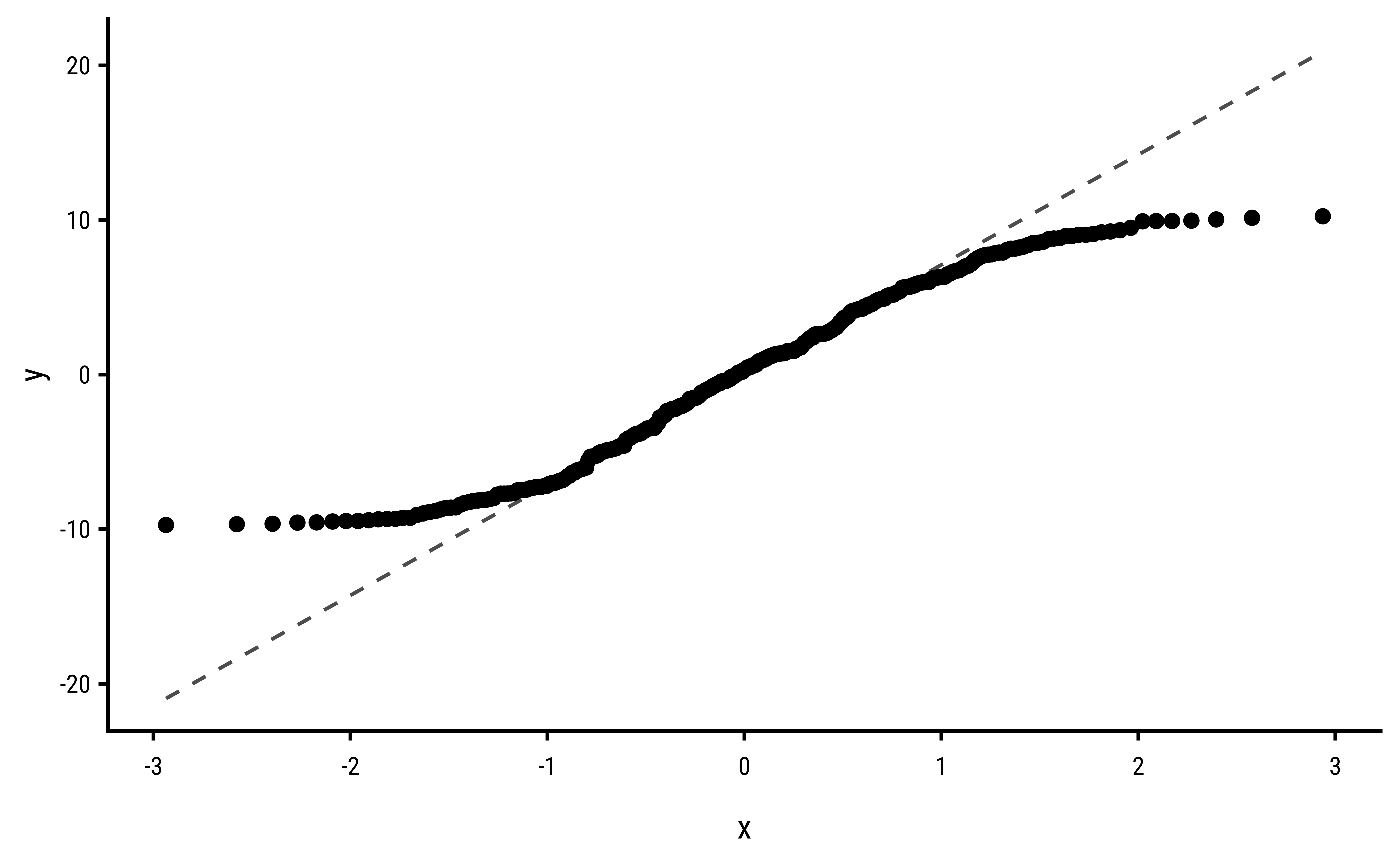
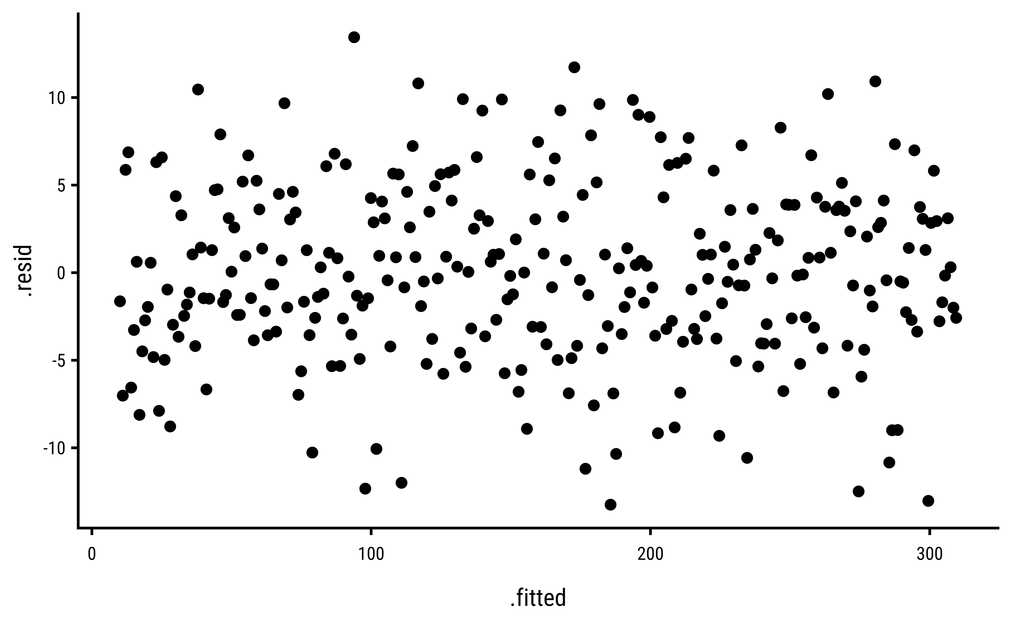
3.2 Uniform Errors

lm_unif_aug <- lm(yu ~ x, data = data) %>%
  augment()
lm_unif_aug %>% gf_point(.resid ~ .fitted)

lm_unif_aug %>%
  gf_qq(~.resid, distribution = stats::qnorm) %>%
  gf_qqline()

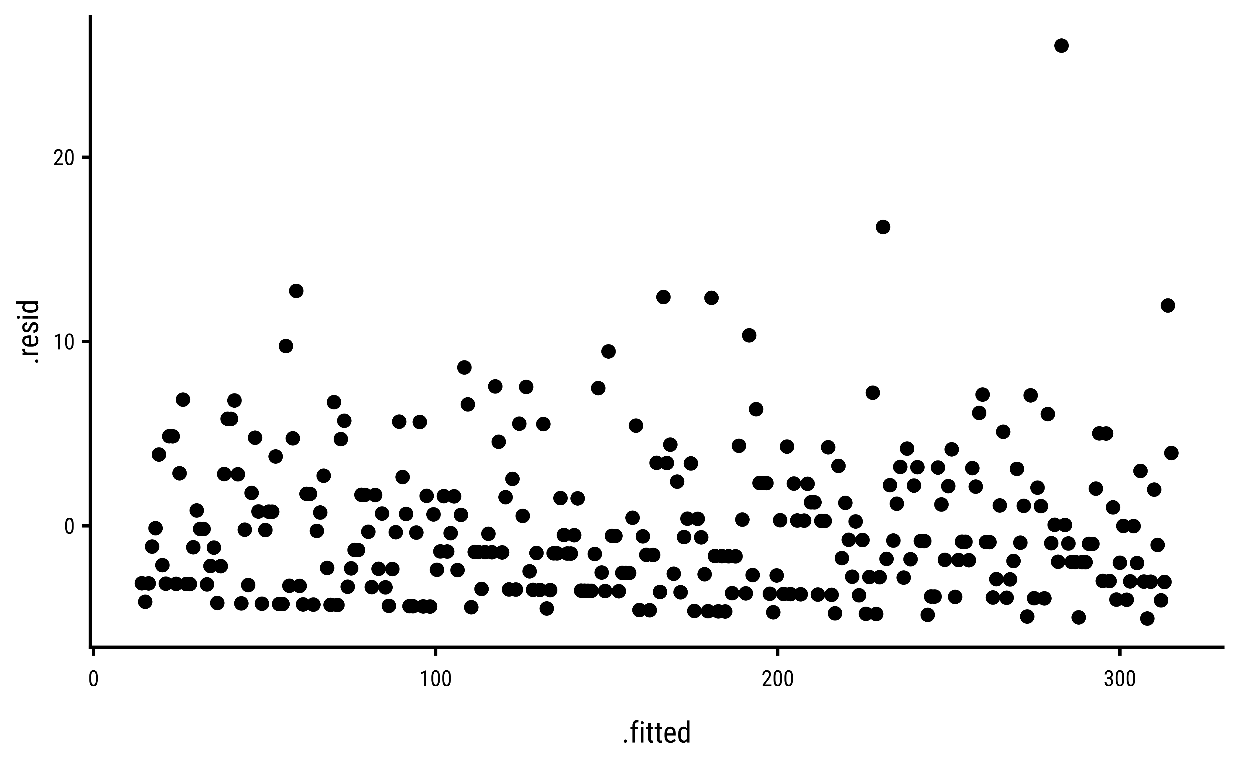
3.3 Negative Binom Errors

lm_nbinom_aug <- lm(yb ~ x, data = data) %>%
  augment()
lm_nbinom_aug %>% gf_point(.resid ~ .fitted)

lm_nbinom_aug %>%
  gf_qq(~.resid, distribution = stats::qnorm) %>%
  gf_qqline()

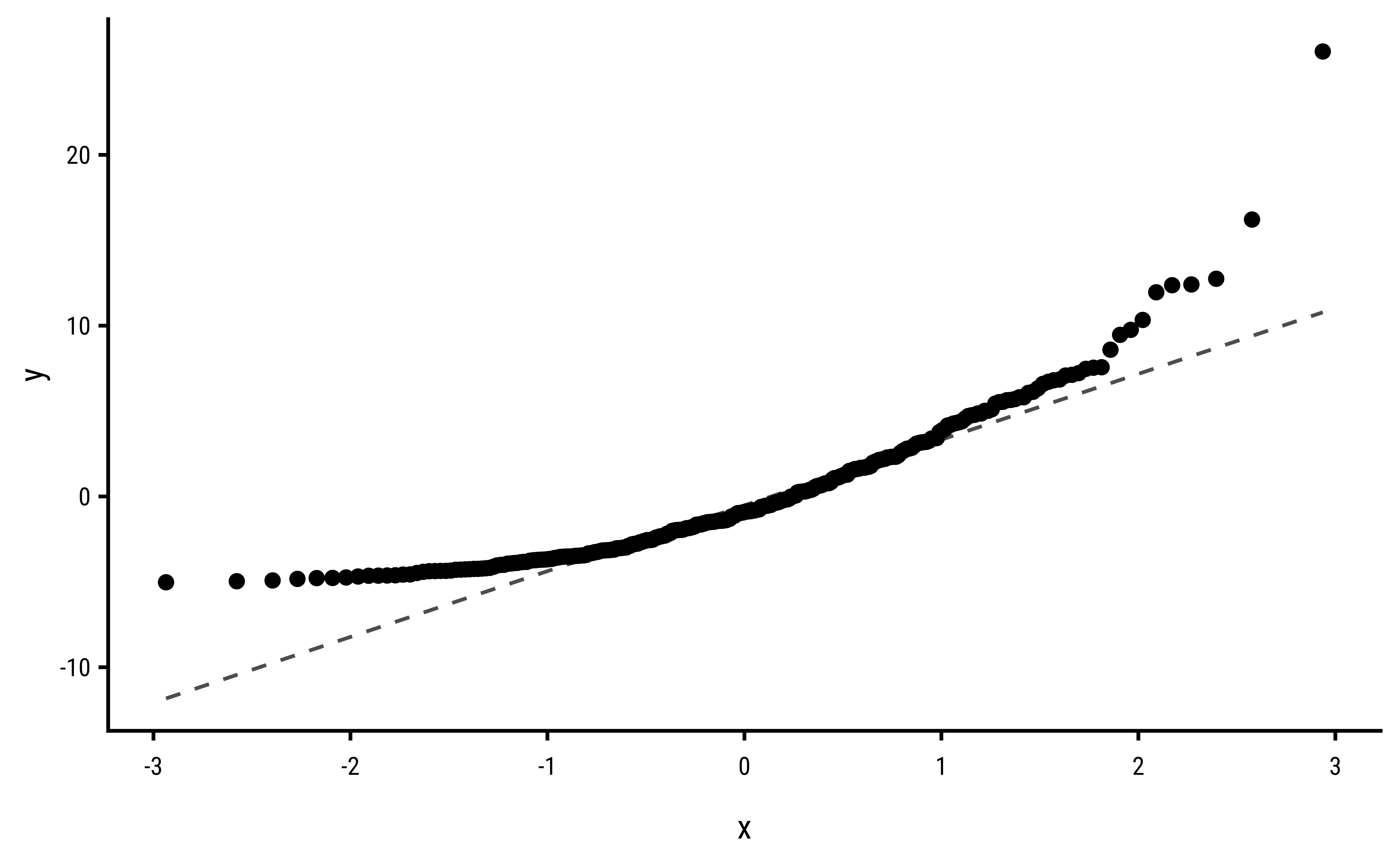
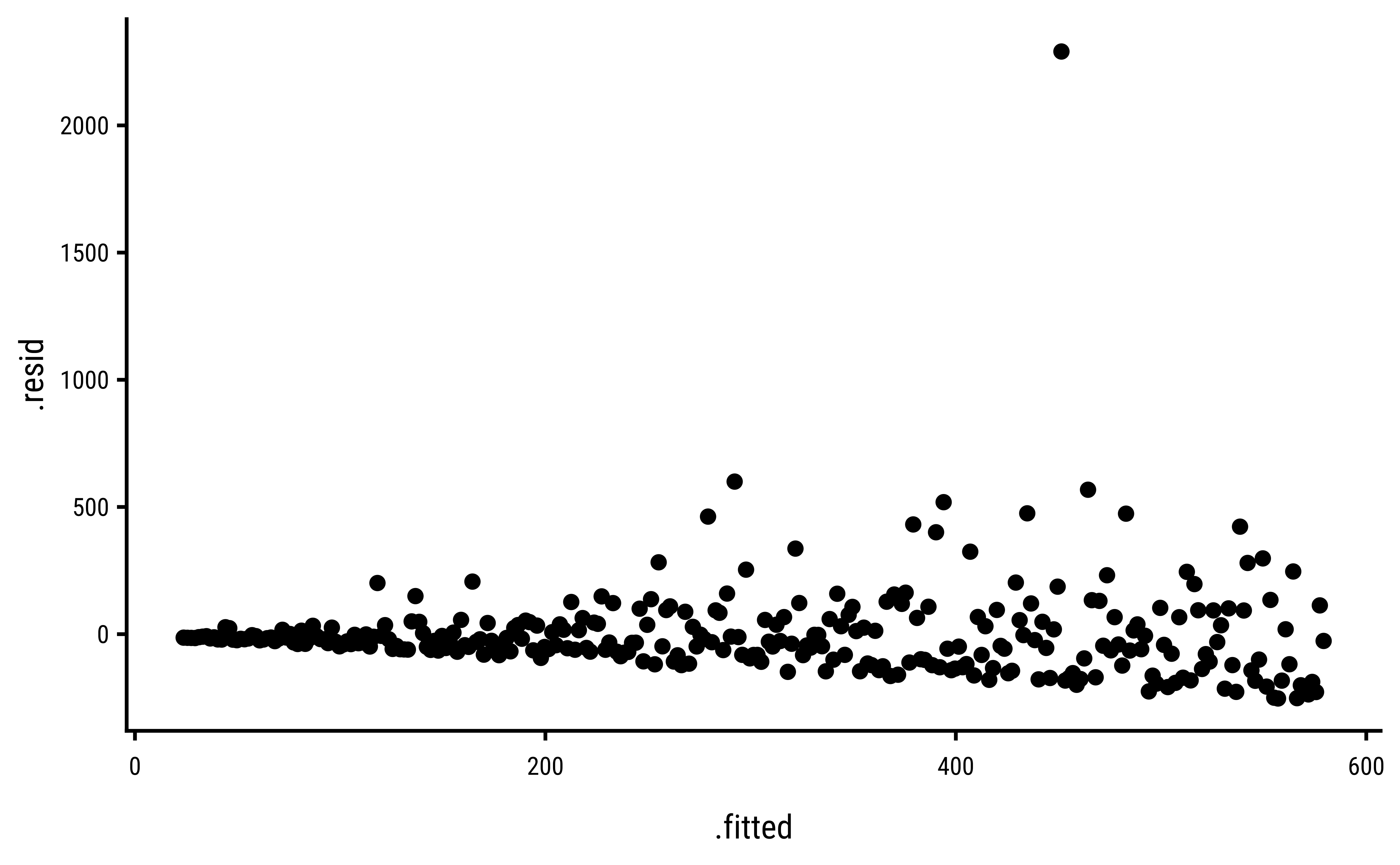
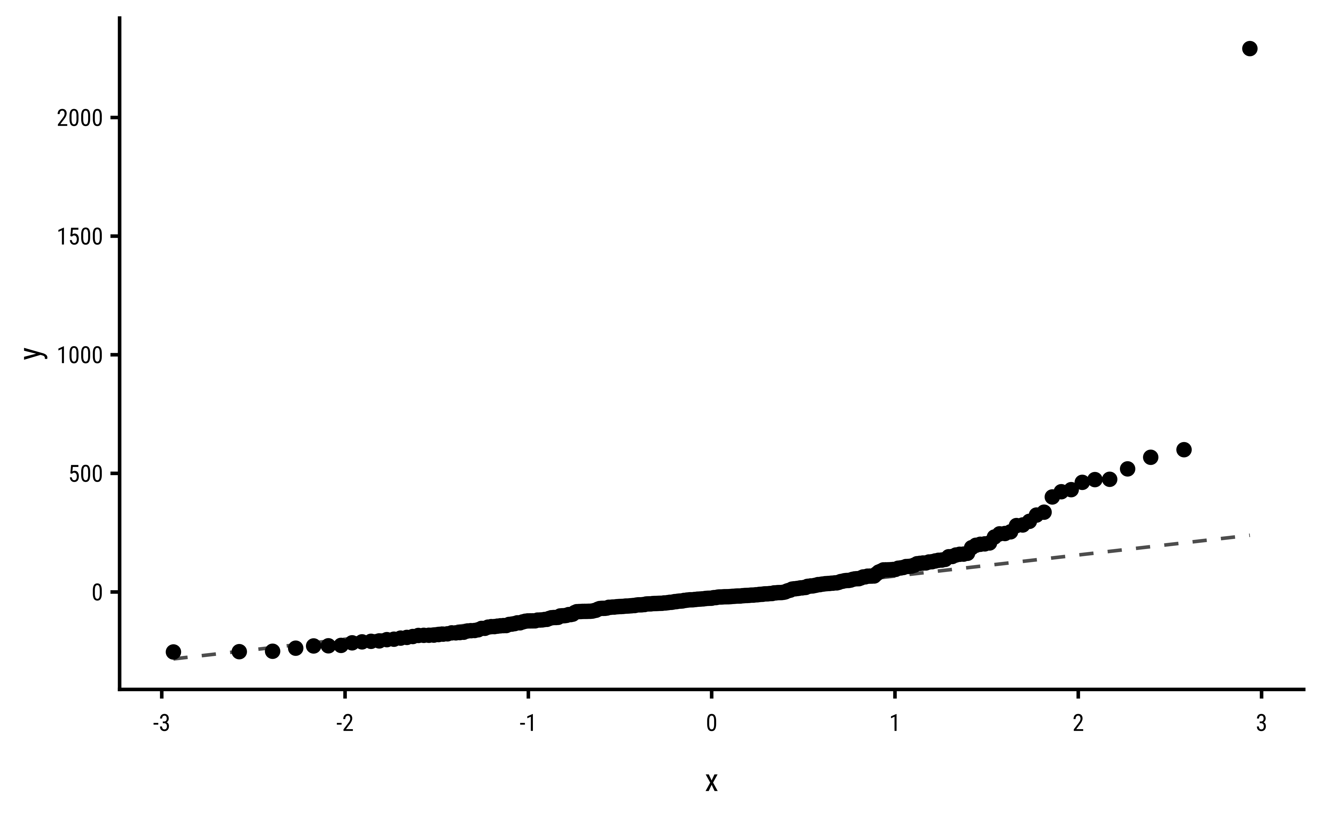
3.4 Gamma Errors

lm_gamm_aug <- lm(yg ~ x, data = data) %>%
  augment()
lm_gamm_aug %>% gf_point(.resid ~ .fitted)

lm_gamm_aug %>%
  gf_qq(~.resid, distribution = stats::qnorm) %>%
  gf_qqline()

Back to top

License: CC BY-SA 2.0

Website made with ❤️ and Quarto, by Arvind V.

Hosted by Netlify .