Data Carpentry

Introduction to the dplyr package

Author

Arvind V.

Published

July 6, 2021

Modified

September 30, 2025

1 Introduction

One of the dominant paradigms of working with data in R is to render it into “tidy” form. A huge benefit of the tidy way of working is that it influences your thinking with data and helps plan out your operations, in going from purpose to actual code in a swift and intuitive manner. This tidy form allows for a huge variety of data manipulation, summarizing, and plotting tasks, that can be performed using the packages of the tidyverse, and other packages that leverage the power of the tidyverse.

2 Setting up the Packages

knitr::opts_chunk$set(message = TRUE) # Want tidylog messages
library(tidyverse)
library(tidylog) ## Explains what happens with dplyr verbs

Plot Fonts and Theme

Show the Code

library(systemfonts)
library(showtext)
library(ggrepel)
library(marquee)
## Clean the slate
systemfonts::clear_local_fonts()
systemfonts::clear_registry()
##
showtext_opts(dpi = 96) # set DPI for showtext
sysfonts::font_add(
  family = "Alegreya",
  regular = "../../../../../../fonts/Alegreya-Regular.ttf",
  bold = "../../../../../../fonts/Alegreya-Bold.ttf",
  italic = "../../../../../../fonts/Alegreya-Italic.ttf",
  bolditalic = "../../../../../../fonts/Alegreya-BoldItalic.ttf"
)

sysfonts::font_add(
  family = "Roboto Condensed",
  regular = "../../../../../../fonts/RobotoCondensed-Regular.ttf",
  bold = "../../../../../../fonts/RobotoCondensed-Bold.ttf",
  italic = "../../../../../../fonts/RobotoCondensed-Italic.ttf",
  bolditalic = "../../../../../../fonts/RobotoCondensed-BoldItalic.ttf"
)
showtext_auto(enable = TRUE) # enable showtext
##
theme_custom <- function() {
  theme_bw(base_size = 10) +

    theme_sub_axis(
      title = element_text(
        family = "Roboto Condensed",
        size = 8
      ),
      text = element_text(
        family = "Roboto Condensed",
        size = 6
      )
    ) +

    theme_sub_legend(
      text = element_text(
        family = "Roboto Condensed",
        size = 6
      ),
      title = element_text(
        family = "Alegreya",
        size = 8
      )
    ) +

    theme_sub_plot(
      title = element_text(
        family = "Alegreya",
        size = 14, face = "bold"
      ),
      title.position = "plot",
      subtitle = element_text(
        family = "Alegreya",
        size = 10
      ),
      caption = element_text(
        family = "Alegreya",
        size = 6
      ),
      caption.position = "plot"
    )
}

## Use available fonts in ggplot text geoms too!
ggplot2::update_geom_defaults(geom = "text", new = list(
  family = "Roboto Condensed",
  face = "plain",
  size = 3.5,
  color = "#2b2b2b"
))
ggplot2::update_geom_defaults(geom = "label", new = list(
  family = "Roboto Condensed",
  face = "plain",
  size = 3.5,
  color = "#2b2b2b"
))

ggplot2::update_geom_defaults(geom = "marquee", new = list(
  family = "Roboto Condensed",
  face = "plain",
  size = 3.5,
  color = "#2b2b2b"
))
ggplot2::update_geom_defaults(geom = "text_repel", new = list(
  family = "Roboto Condensed",
  face = "plain",
  size = 3.5,
  color = "#2b2b2b"
))
ggplot2::update_geom_defaults(geom = "label_repel", new = list(
  family = "Roboto Condensed",
  face = "plain",
  size = 3.5,
  color = "#2b2b2b"
))

## Set the theme
ggplot2::theme_set(new = theme_custom())

## tinytable options
options("tinytable_tt_digits" = 2)
options("tinytable_format_num_fmt" = "significant_cell")
options(tinytable_html_mathjax = TRUE)


## Set defaults for flextable
flextable::set_flextable_defaults(font.family = "Roboto Condensed")

3 Tidy Data

“Tidy Data” is an important way of thinking about what data typically look like in R. Let’s fetch a figure from the web to show the (preferred) structure of data in R.

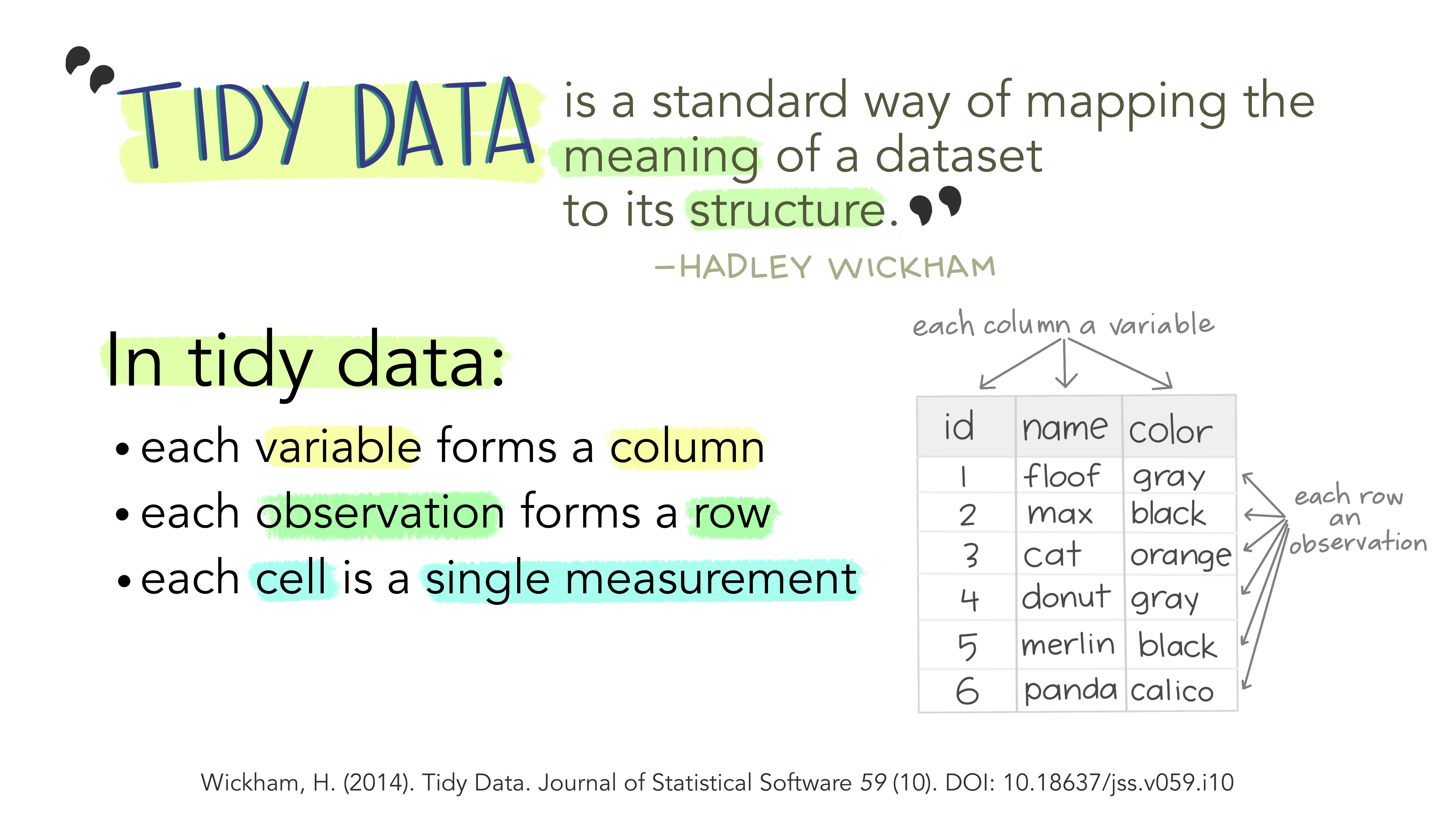
The three features described in the figure above define the nature of tidy data:

Variables in Columns
Observations in Rows and
Measurements in Cells.

Data are imagined to be resulting from an experiment. Each variable represents a parameter/aspect in the experiment. Each row represents an additional datum of measurement. A cell is a single measurement on a single parameter(column) in a single observation(row).

When working with data you must:

Figure out what you want to do. (Purpose)
Describe those tasks in the form of a computer program. (Plain English to R Code)
Execute the program.

The dplyr package makes these steps fast and easy:

By constraining your options, it helps you think about your data manipulation challenges.
It provides simple “verbs”, functions that correspond to the most common data manipulation tasks, to help you translate your thoughts into code.
It uses efficient backends, so you spend less time waiting for the computer.

Shakespeare on Backends

Ne’er you mind about backends ;-) See Shakespeare’s Hamlet.

This document introduces you to dplyr’s basic set of tools, and shows you how to apply them to data frames.

4 Data: starwars

We will play with the starwars dataset that comes with the dplyr.

data(starwars)
dim(starwars)

[1] 87 14

starwars

To explore the basic data manipulation verbs of dplyr, we’ll use the dataset starwars. This dataset contains 87 characters and comes from the Star Wars API, and is documented in ?starwars.

This means: type ?starwars in the Console. Try.

Note that starwars is a tibble, a modern re-imagining of the data frame. It’s particularly useful for large datasets because it only prints the first few rows. You can learn more about tibbles at https://tibble.tidyverse.org; in particular you can convert data frames to tibbles with as_tibble().

Check your Environment Tab to inspect starwars in a separate tab.

5 Single table verbs

dplyr aims to provide a function for each basic verb of data manipulation. These verbs can be organised into three categories based on the component of the dataset that they work with:

Rows:
- dplyr::filter() chooses rows based on column values.
- dplyr::slice() chooses rows based on location.
- dplyr::arrange() changes the order of the rows.
Columns:
- dplyr::select() changes whether or not a column is included.
- dplyr::rename() changes the name of columns.
- dplyr::mutate() changes the values of columns and creates new columns.
- dplyr::relocate() changes the order of the columns.
Groups of rows:
- dplyr::summarise() collapses a group into a single row.

Think of the parallels from Microsoft Excel.

5.1 The pipe

All of the dplyr functions take a data frame (or tibble) as the first argument. Rather than forcing the user to either save intermediate objects or nest functions, dplyr provides the pipe %>% operator from the package magrittr. x %>% f(y) turns into f(x, y) so the result from one step is then “piped” into the next step. You can use the pipe to rewrite multiple operations that you can read left-to-right, top-to-bottom (reading the pipe operator as “then”).

5.2 Filter rows with `filter()`

filter() allows you to select a subset of rows in a data frame. Like all single verbs, the first argument is the tibble (or data frame). The second and subsequent arguments refer to variables within that data frame, selecting rows where the expression is TRUE.

For example, we can select all character with light skin color and brown eyes with:

Important

Note the double equal to sign (==) below! Equivalent to MS Excel Data -> Filter.

starwars %>%
  dplyr::filter(skin_color == "light", eye_color == "brown")

5.3 Arrange rows with `arrange()`

arrange() works similarly to filter() except that instead of filtering or selecting rows, it reorders them. It takes a data frame, and a set of column names (or more complicated expressions) to order by. If you provide more than one column name, each additional column will be used to break ties in the values of preceding columns:

starwars %>% dplyr::arrange(height, mass)

Use desc() to order a column in descending order:

starwars %>% dplyr::arrange(desc(height))

5.4 Choose rows using their position with `slice()`

slice() lets you index rows by their (integer) locations. It allows you to select, remove, and duplicate rows.

Tip

This is an important step in Prediction, Modelling and Machine Learning.

We can get characters from row numbers 5 through 10.

starwars %>% dplyr::slice(5:10)

It is accompanied by a number of helpers for common use cases:

slice_head() and slice_tail() select the first or last rows.

starwars %>% dplyr::slice_head(n = 3)

slice_sample() randomly selects rows. Use the option prop to choose a certain proportion of the cases.

starwars %>% dplyr::slice_sample(n = 5)

starwars %>% dplyr::slice_sample(prop = 0.1)

Use replace = TRUE to perform a bootstrap sample. If needed, you can weight the sample with the weight argument.

Selecting with Replacement = “Bootstrap”

Bootstrap samples are a special statistical sampling method. Counter-intuitive perhaps, since you sample with replacement. Should remind you of your high school Permutation and Combination class, with all those urn models and so on. If you remember.

slice_min() and slice_max() select rows with highest or lowest values of a variable. Note that we first must choose only the values which are not NA.

starwars %>%
  dplyr::filter(!is.na(height)) %>%
  dplyr::slice_min(height, n = 3)

5.5 Select columns with `select()`

Often you work with large datasets with many columns but only a few are actually of interest to you. select() allows you to rapidly zoom in on a useful subset using operations that usually only work on numeric variable positions:

# Select columns by name
starwars %>% dplyr::select(hair_color, skin_color, eye_color)

# Select all columns between hair_color and eye_color (inclusive)
starwars %>% dplyr::select(hair_color:eye_color)

# Select all columns except those from hair_color to eye_color (inclusive)
starwars %>% dplyr::select(!(hair_color:eye_color))

# Select all columns ending with color
starwars %>% dplyr::select(ends_with("color"))

There are a number of helper functions you can use within select(), like starts_with(), ends_with(), matches() and contains(). These let you quickly match larger blocks of variables that meet some criterion. See ?select for more details.

You can rename variables with rename()` by using named arguments:

starwars %>% dplyr::rename(home_world = homeworld)

5.6 Add new columns with `mutate()`

Besides selecting sets of existing columns, it’s often useful to add new columns that are functions of existing columns. This is the job of mutate():

starwars %>% dplyr::mutate(height_m = height / 100)

We can’t see the height in meters we just calculated, but we can fix that using a select command.

starwars %>%
  dplyr::mutate(height_m = height / 100) %>%
  dplyr::select(height_m, height, everything())

dplyr::mutate() even allows you to refer to columns that you’ve just created:

starwars %>%
  dplyr::mutate(
    height_m = height / 100,
    BMI = mass / (height_m^2)
  ) %>%
  dplyr::select(BMI, everything())

If you only want to keep the new variables, use transmute():

starwars %>%
  dplyr::transmute(
    height_m = height / 100,
    BMI = mass / (height_m^2)
  )

5.7 Change column order with `relocate()`

Use a similar syntax as select() to move blocks of columns at once

starwars %>% dplyr::relocate(sex:homeworld, .before = height)

5.8 Summarise values with `summarise()`

The last verb is summarise(). It collapses a data frame to a single row.

starwars %>%
  dplyr::summarise(mean_height = mean(height, na.rm = TRUE))

It’s not that useful until we learn the group_by() verb below.

5.9 Commonalities

You may have noticed that the syntax and function of all these verbs are very similar:

The first argument is a data frame.
The subsequent arguments describe what to do with the data frame. You can refer to columns in the data frame directly by name.
The result is a new data frame

Together these properties make it easy to chain together multiple simple steps to achieve a complex result.

These five functions provide the basis of a language of data manipulation. At the most basic level, you can only alter a tidy data frame in five useful ways: you can reorder the rows (arrange()), pick observations and variables of interest (filter() and select()), add new variables that are functions of existing variables (mutate()), or collapse many values to a summary (summarise()).

6 Combining functions with `%>%`

dplyr provides the %>% operator from magrittr. x %>% f(y) turns into f(x, y) so you can use it to rewrite multiple operations that you can read left-to-right, top-to-bottom (reading the pipe operator as “then”):

starwars %>%
  group_by(species, sex) %>%
  summarise(
    mean_height = mean(height, na.rm = TRUE),
    mean_mass = mean(mass, na.rm = TRUE)
  )

group_by: 2 grouping variables (species, sex)
summarise: now 41 rows and 4 columns, one group variable remaining (species)

7 Patterns of operations

The dplyr verbs can be classified by the type of operations they accomplish (we sometimes speak of their semantics, i.e., their meaning). It’s helpful to have a good grasp of the difference between select and mutate operations.

7.1 Selecting operations

One of the appealing features of dplyr is that you can refer to columns from the tibble as if they were regular variables. Selecting operations expect column names and positions. Hence, when you call select() with bare variable names, they actually represent their own positions in the tibble. The following calls are completely equivalent from dplyr’s point of view:

# `name` is the first column in the tibble
dplyr::select(starwars, name)

dplyr::select(starwars, 1)

7.2 Mutating operations

Mutate semantics are quite different from selection semantics. Whereas select() expects column names or positions, mutate() expects the actual data, the column vectors themselves. We will set up a smaller tibble to use for our examples.

df <- starwars %>% dplyr::select(name, height, mass)

When we use select(), the bare column names stand for their own positions in the tibble. For mutate() on the other hand, column symbols represent the actual column vectors stored in the tibble. Consider what happens if we wish to add a number to all entries in a column using mutate(): The correct expression is:

dplyr::mutate(df, height + 10)

Here inside mutate(), the symbol height represents the actual column, whereas in select(), it represents the position of the column. This is a crucial difference.

Another case in point is group_by(). While you might think it has select semantics, it actually has mutate semantics. This is quite handy as it allows to group by a modified column:

group_by(starwars, sex)

group_by: one grouping variable (sex)

group_by(starwars, sex = as.factor(sex))

group_by: one grouping variable (sex)

group_by(starwars, height_binned = cut(height, 3))

group_by: one grouping variable (height_binned)

8 Two table verbs

Sometimes our data is spread across more than one table. Often these tables are linked by some common, or common-looking, variable columns. dplyr allows us to work with such data that is spread over more than one table. More information is available here: Two Table Verbs in dplyr

The operations/verbs used to manipulate two-table verbs are:

Mutating joins, which add new variables to one table from matching rows in another.
- inner_join()

left_join()

right_join()

full_join()

Filtering joins, which filter observations from one table based on whether or not they match an observation in the other table.
semi_join(x, y) keeps all observations in x that have a match in y.

anti_join(x, y) drops all observations in x that have a match in

Set operations, which combine the observations in the data sets as if they were set elements.
- union()

-   union_all(),

-   intersect(),

setdiff()

Tidyr Operations:
pivot_longer()
pivot_wider()

We will examine these when we actually need to use them !!!

9 Conclusion

This module introduced you to the dplyr package, which provides a set of verbs that help you solve the most common data manipulation challenges. The five main verbs are:

dplyr::filter(): pick rows by their values
dplyr::arrange(): reorder rows
dplyr::select(): pick columns by their names (and helpers)
dplyr::mutate(): create new columns
dplyr::group_by(): group rows by the values of a column
dplyr::summarise(): collapse many values down to a single summary

We also saw rename and relocate briefly, and transmute in passing.

These verbs can be combined using the pipe operator %>% to express complex operations in a clear and concise way.

1 Introduction

2 Setting up the Packages

Plot Fonts and Theme

3 Tidy Data

4 Data: starwars

5 Single table verbs

5.1 The pipe

5.2 Filter rows with filter()

5.3 Arrange rows with arrange()

5.4 Choose rows using their position with slice()

5.5 Select columns with select()

5.6 Add new columns with mutate()

5.7 Change column order with relocate()

5.8 Summarise values with summarise()

5.9 Commonalities

6 Combining functions with %>%

7 Patterns of operations

7.1 Selecting operations

7.2 Mutating operations

8 Two table verbs

9 Conclusion

5.2 Filter rows with `filter()`

5.3 Arrange rows with `arrange()`

5.4 Choose rows using their position with `slice()`

5.5 Select columns with `select()`

5.6 Add new columns with `mutate()`

5.7 Change column order with `relocate()`

5.8 Summarise values with `summarise()`

6 Combining functions with `%>%`