1 Setting up R Packages
2 Introduction
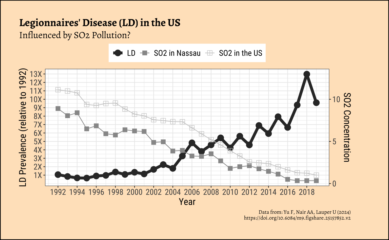
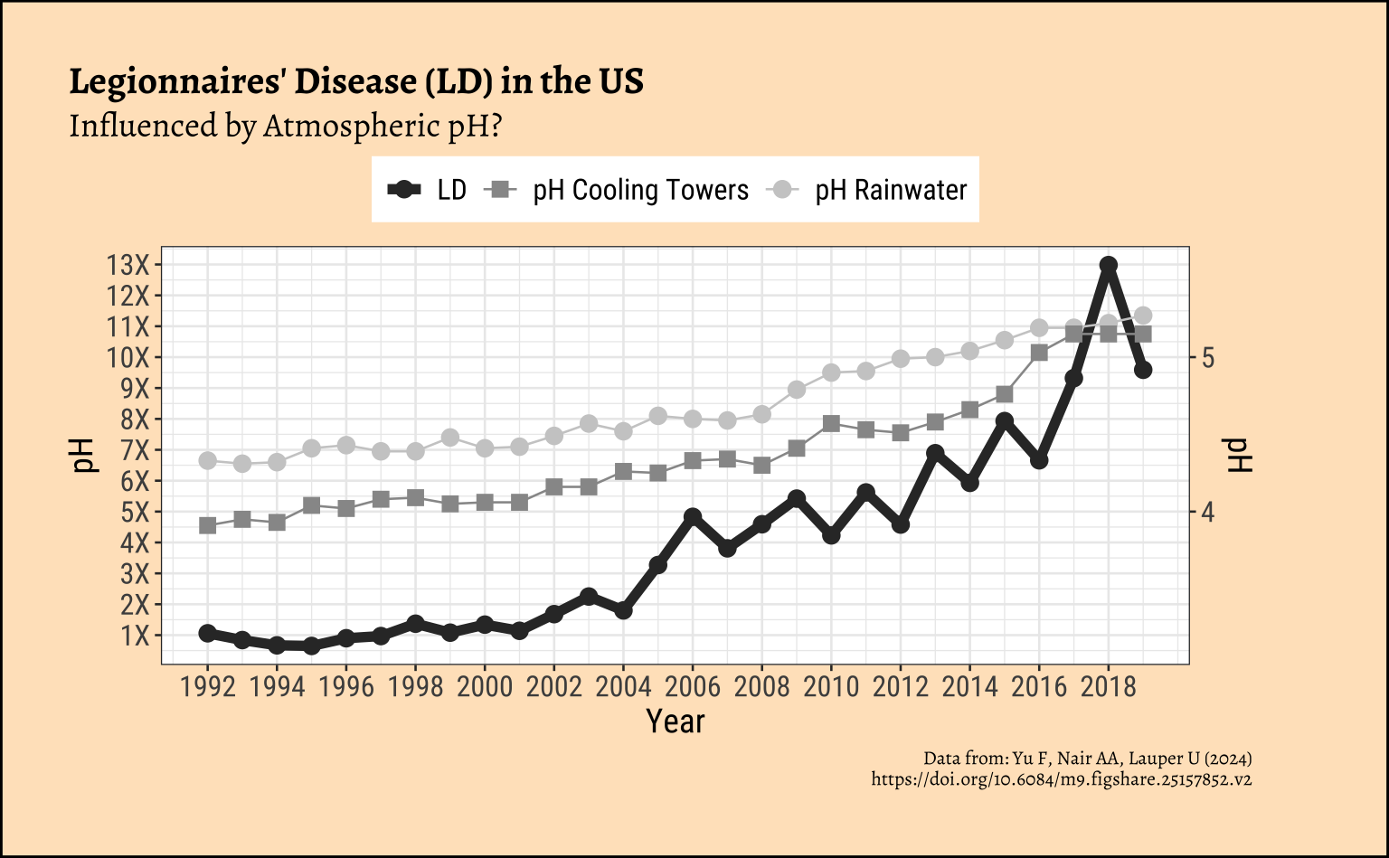
Legionnaires’ disease (LD) is a severe form of pneumonia (∼10–25% fatality rate) caused by inhalation of aerosols containing Legionella, a pathogenic gram-negative bacteria. These bacteria can grow, spread, and aerosolize through building water systems. A recent dramatic increase in LD incidence has been observed globally, with a 9-fold increase in the United States from 2000 to 2018,
Records were also maintained of atmospheric Sulphur Dioxide (SO2) and the acidity i.e. pH of the atmosphere around building water systems such as Cooling Towers (CT) and in Rainwater.
This data is from this paper: Yu F, Nair AA, Lauper U (2024), https://doi.org/10.6084/m9.figshare.25157852.v2
3 Read the Modified Data
4 Inspect the Data
```{r}
#| label: inspect-skim-glimpse

# Write in
```
5 Data Dictionary
Write in.
Write in.
Write in.
Describe how you may plan to transform the data.
6 Research Question
Write in! Look first at the Charts below!
7 Join the Data
```{r}
#| label: data-preprocessing
#
# Write in your code here
# to prepare this data as shown below
# to generate the plot that follows
```
Here is the plot-ready data:
8 Plot the Data
Two plots were generated by the researchers with this data. Can you reproduce these? Do these graphs prove/disprove any of your hypotheses? What might have been the Hypotheses that led the creating of these graphs?
Show the Code
ld_mod %>%
  gf_line(ld ~ year,
    linewidth = 2,
    xlab = "Year",
    title = "Legionnaires' Disease (LD) in the US",
    colour = ~"LD",
    subtitle = "Influenced by SO2 Pollution?",
    caption = "Data from: Yu F, Nair AA, Lauper U (2024)\n https://doi.org/10.6084/m9.figshare.25157852.v2"
  ) %>%
  gf_point(
    ylab = "LD Prevalence (relative to 1992)",
    colour = ~"LD", size = 4
  ) %>%
  gf_line(so2_Nassau_Erie ~ year,
    colour = ~"SO2 in Nassau"
  ) %>%
  gf_point(so2_Nassau_Erie ~ year,
    colour = ~"SO2 in Nassau",
    shape = 15, size = 3
  ) %>%
  gf_line(so2_US ~ year, colour = ~"SO2 in the US") %>%
  gf_point(so2_US ~ year,
    colour = ~"SO2 in the US",
    shape = 12, size = 3
  ) %>%
  gf_refine(
    scale_colour_grey("LD"),
    scale_x_continuous(breaks = seq(1992, 2019, 2)),
    ## Ratiometric Y-scale
    scale_y_continuous(
      breaks = seq(1:15),
      labels = scales::label_number(
        scale = 1,
        suffix = "X"
      ),
      sec.axis = sec_axis(
        trans = ~ . / 1,
        name = "SO2 Concentration"
      )
    )
  ) %>%
  gf_theme(theme(
    legend.title = element_blank(),
    legend.position = "top"
  ))
Show the Code
ld_mod %>%
  gf_line(ld ~ year,
    linewidth = 2,
    xlab = "Year",
    colour = ~"LD"
  ) %>%
  gf_point(
    ylab = "LD Prevalence (relative to 1992)",
    colour = ~"LD", size = 3
  ) %>%
  gf_line(5 * (pH_rainwater - 3) ~ year,
    colour = ~"pH Rainwater"
  ) %>%
  gf_point(5 * (pH_rainwater - 3) ~ year,
    colour = ~"pH Rainwater", size = 3
  ) %>%
  gf_line(5 * (pH_CT - 3) ~ year,
    colour = ~"pH Cooling Towers",
    ylab = "pH"
  ) %>%
  gf_point(
    5 * (pH_CT - 3) ~ year,
    colour = ~"pH Cooling Towers",
    shape = 15,
    size = 3
  ) %>%
  gf_refine(
    scale_colour_grey("pH"),
    scale_x_continuous(breaks = seq(1992, 2019, 2)),
    scale_y_continuous(
      breaks = seq(1:15),
      labels = scales::label_number(
        scale = 1,
        suffix = "X"
      ),
      sec.axis = sec_axis(
        trans = ~ (.x / 5 + 3),
        name = "pH"
      )
    )
  ) %>%
  gf_labs(
    title = "Legionnaires' Disease (LD) in the US",
    subtitle = "Influenced by Atmospheric pH?",
    caption = "Data from: Yu F, Nair AA, Lauper U (2024)\n https://doi.org/10.6084/m9.figshare.25157852.v2"
  ) %>%
  gf_theme(theme(
    legend.title = element_blank(),
    legend.position = "top"
  ))
9 Tasks and Discussion
- Complete the Data Dictionary.
- Select and Transform the variables as shown. Combine the multiple datasets into one if needed!
- Create the graphs shown and discuss the following questions:
- Identify the type of charts
- Identify the variables used for various geometrical aspects (x, y, fill…). Name the variables appropriately.
- What is a peculiar feature of these graphs?
- What might have been the Hypothesis/Research Question to which the response was Chart?
- What data gathering / research activity might have been carried out to obtain the data graphed here? Provide some details.
- Write a short story based on the chart, describing your inference/surprise.
- Is there a paradox in this case study? Hint: SO2 is caused by cars/busses running on fossil fuels.
- What Statistical Tests might you run to confirm what the charts are saying?